
计算机视觉:Harris角点检测与SIFT特征提取
计算机视觉:Harris角点检测与SIFT特征提取
文章目录
1实验内容:
1.分别实现Harris角点检测与SIFT特征提取,对比两者的区别
2.利用SIFT算法实现两幅相近图像的特征匹配
3.实现匹配地理标记图像
1.Harris角点检测算法的原理以及实现
1)原理及理解
1、角点的概念:
如果一个点在任意方向的一个微小变动都会引起灰度很大的变化,那么我们就把它称之为角点,也就是一阶导数(即灰度图的梯度)中的局部最大所对应的像素点就是角点。在现实世界中,角点对应于物体的拐角,道路的十字路口、丁字路口等。基于图像灰度的方法通过计算点的曲率及梯度来检测角点。
2.Harris角点检测的原理:
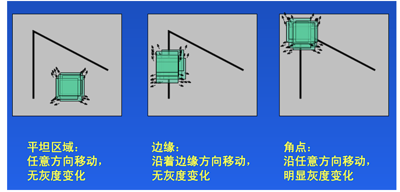
Harris角点检测的思想是通过图像的局部的小窗口观察图像,角点的特征是窗口沿任意方向移动都会导致图像灰度的明显变化,如下图所示:
其数学原理形式表示为

其中:[u,v]是窗口WW的偏移量;(x,y)是窗口W所对应的像素坐标位置,窗口有多大,就有多少个位置;I(x,y)是像素坐标位置(x,y)的图像灰度值;I(x+u,y+v)是像素坐标位置(x+u,y+v)的图像灰度值;w(x,y)是窗口函数,最简单情形就是窗口W内的所有像素所对应的w权重系数均为1,窗口外都为0.但有时候,我们会将w(x,y)函数设置为以窗口W中心为原点的二元正太分布。如果窗口W中心点是角点时,移动前与移动后,该点在灰度变化贡献最大;而离窗口W中心(角点)较远的点,这些点的灰度变化几近平缓,这些点的权重系数,可以设定小值,以示该点对灰度变化贡献较小,那么我们自然使用二元高斯函数来表示窗口函数;
对表达式进行泰勒展开与化简之后得到
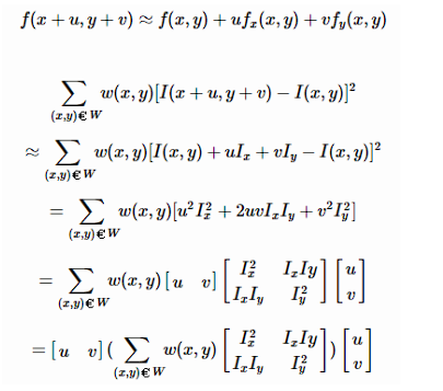
E(u,v)表达式可以化简为:
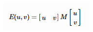

M矩阵决定了E(u,v)的取值,下面我们利用M来求角点,M是Ix 和Iy的二次项函数,可以表示成椭圆的形状,椭圆的长短半轴由M的特征值λ1和λ2决定,方向由特征矢量决定,如下图所示:
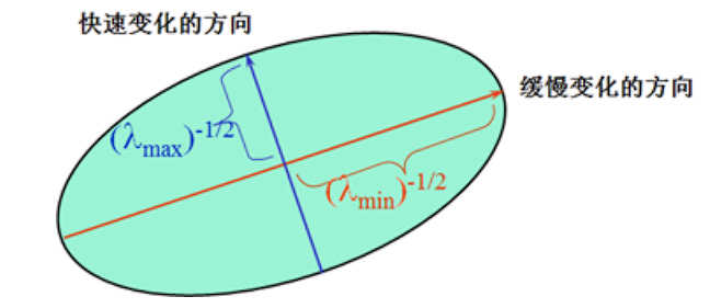
椭圆函数特征值与图像中的角点、直线(边缘)和平面之间的关系如下图所示。
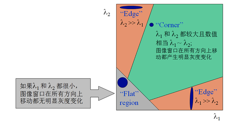
共可分为三种情况:
- 图像中的直线。一个特征值大,另一个特征值小,λ1>>λ2或 λ2>>λ1。椭圆函数值在某一方向上大,在其他方向上小。
- 图像中的平面。两个特征值都小,且近似相等;椭圆函数数值在各个方向上都小。
- 图像中的角点。两个特征值都大,且近似相等,椭圆函数在所有方向都增大
Harris给出的角点计算方法并不需要计算具体的特征值,而是计算一个角点响应值R来判断角点。R的计算公式为:
式中,detM为矩阵M的行列式;traceM为矩阵M的迹;α为常数,取值范围为0.04~0.06。事实上,特征是隐含在detM和traceM中,因为: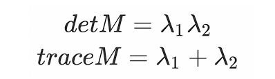
那我们怎么判断角点呢?如下图所示:
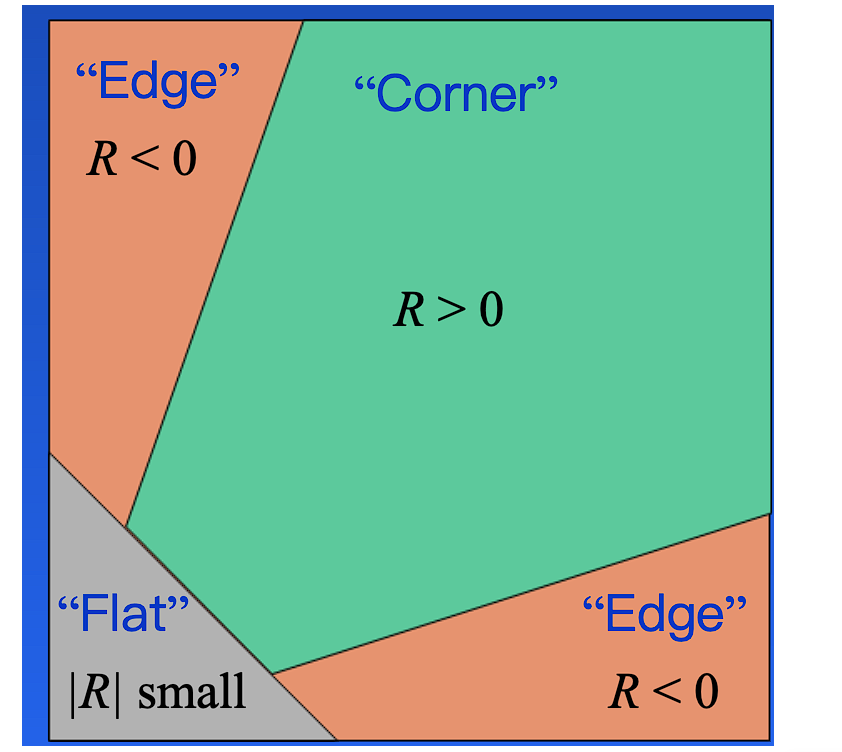
- 当R为大数值的正数时是角点
- 当R为大数值的负数时是边界
- 当R为小数是认为是平坦区域
在OpenCV中实现Hariis检测使用的API是:
dst=cv.cornerHarris(src, blockSize, ksize, k)
参数:
- img:数据类型为 float32 的输入图像。
- blockSize:角点检测中要考虑的邻域大小。
- ksize:sobel求导使用的核大小
- k :角点检测方程中的自由参数,取值参数为 [0.04,0.06].
2)实现
opencv库函数cv.cornerHarris()实现
import cv2 as cv
import numpy as np
import matplotlib.pyplot as plt


img = cv.imread('./ex2/cornertest.jpg')
gray = cv.cvtColor(img, cv.COLOR_BGR2GRAY)
gray = np.float32(gray)
dst = cv.cornerHarris(gray,2,3,0.04)
#阈值设置
img[dst>0.001*dst.max()] = [0,0,255]

plt.figure(figsize=(10,8),dpi=100)
plt.imshow(img[:,:,::-1]),plt.title('Harris')
plt.xticks([]), plt.yticks([])
plt.show()
实验结果:
原图像:
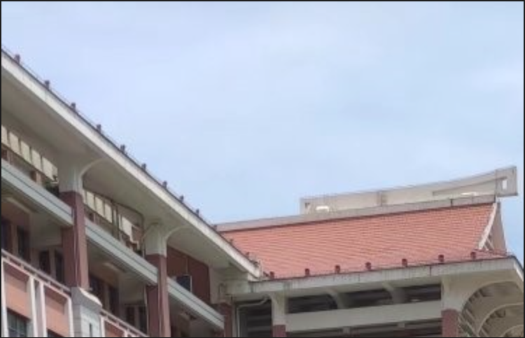
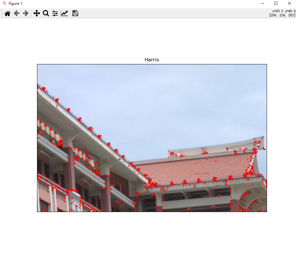
阈值=0.001,harris算法效果
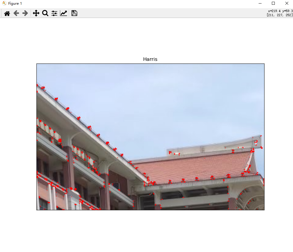
阈值=0.01,harris算法效果:
阈值=0.1,harris算法效果
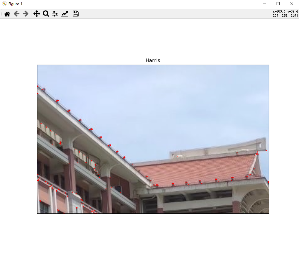
在进行角点检测时,随着阈值变大,能被检测到的角点会相应的减少
2.利用SIFT算法实现两幅相近图像的特征匹配
1原理及理解
2)实现
import cv2
import numpy as np
import matplotlib.pyplot as plt


img1 = cv2.imread('./ex2/sift1.jpg')
img2 = cv2.imread('./ex2/sift2.jpg')

img1 = cv2.cvtColor(img1, cv2.COLOR_BGR2RGB)
img2 = cv2.cvtColor(img2, cv2.COLOR_BGR2RGB)


def extract_sift_features(image, num_features):
    # 提取特征点和计算描述符.
    sift_detector = cv2.SIFT_create(num_features, contrastThreshold=-10000, edgeThreshold=-10000)  # 创建一个sift特征检测对象
    gray = cv2.cvtColor(image, cv2.COLOR_RGB2GRAY)
    kp, desc = sift_detector.detectAndCompute(gray, None)  # 用检测器检测关键点并计算描述符
    return kp[:num_features], desc[:num_features]


key_point_1, descriptor_1 = extract_sift_features(img1, 2000)
key_point_2, descriptor_2 = extract_sift_features(img2, 2000)

img_with_kp_1 = cv2.drawKeypoints(img1, key_point_1, outImage=None, flags=cv2.DRAW_MATCHES_FLAGS_DRAW_RICH_KEYPOINTS)
img_with_kp_2 = cv2.drawKeypoints(img2, key_point_2, outImage=None, flags=cv2.DRAW_MATCHES_FLAGS_DRAW_RICH_KEYPOINTS)
print(f'img1 find {len(key_point_1)} features')
print(f'img2 find {len(key_point_2)} features')
fig = plt.figure(figsize=(30, 15))
plt.subplot(121)
plt.imshow(img_with_kp_1)
plt.axis('off')
plt.subplot(122)
plt.imshow(img_with_kp_2)
plt.axis('off')
plt.show()


bf = cv2.BFMatcher(cv2.NORM_L2, crossCheck=True)    # 创建一个L2范数的匹配器
cv_matches = bf.match(descriptor_1, descriptor_2)   # 匹配两个描述子,返回最佳匹配(object)
# 将关键点和匹配点转换成矩阵
matches = np.array([[m.queryIdx, m.trainIdx] for m in cv_matches])
keyarr_1 = np.array([kp.pt for kp in key_point_1])
keyarr_2 = np.array([kp.pt for kp in key_point_2])


def build_composite_image(im1, im2, axis=1, margin=0, background=1):
    '''拼接两张不同尺寸的图片.'''
    # 输入:axis:拼接基准坐标
    # 		margin:间距
    # 		background:背景色
    # 输出:composite:拼接结果;
    # 		(voff1, voff2):左右偏移;
    #		(hoff1, hoff2):上下偏移

    if background != 0 and background != 1:
        background = 1
    if axis != 0 and axis != 1:
        raise RuntimeError('Axis must be 0 (vertical) or 1 (horizontal')

    h1, w1, _ = im1.shape
    h2, w2, _ = im2.shape

    if axis == 1:
        composite = np.zeros((max(h1, h2), w1 + w2 + margin, 3), dtype=np.uint8) + 255 * background
        if h1 > h2:
            voff1, voff2 = 0, (h1 - h2) // 2
        else:
            voff1, voff2 = (h2 - h1) // 2, 0
        hoff1, hoff2 = 0, w1 + margin
    else:
        composite = np.zeros((h1 + h2 + margin, max(w1, w2), 3), dtype=np.uint8) + 255 * background
        if w1 > w2:
            hoff1, hoff2 = 0, (w1 - w2) // 2
        else:
            hoff1, hoff2 = (w2 - w1) // 2, 0
        voff1, voff2 = 0, h1 + margin
    composite[voff1:voff1 + h1, hoff1:hoff1 + w1, :] = im1
    composite[voff2:voff2 + h2, hoff2:hoff2 + w2, :] = im2

    return composite, (voff1, voff2), (hoff1, hoff2)


def draw_matches(im1, im2, kp1, kp2, matches, axis=1, margin=0, background=0, linewidth=2):
    '''绘制匹配.'''

    composite, v_offset, h_offset = build_composite_image(im1, im2, axis, margin, background)

    # Draw all keypoints.
    for coord_a, coord_b in zip(kp1, kp2):
        # 注意坐标系转换,cv画图和np画图坐标系相反。
        composite = cv2.drawMarker(composite, (int(coord_a[0] + h_offset[0]), int(coord_a[1] + v_offset[0])),
                                   color=(255, 0, 0), markerType=cv2.MARKER_CROSS, markerSize=5, thickness=1)
        composite = cv2.drawMarker(composite, (int(coord_b[0] + h_offset[1]), int(coord_b[1] + v_offset[1])),
                                   color=(255, 0, 0), markerType=cv2.MARKER_CROSS, markerSize=5, thickness=1)

    # Draw matches, and highlight keypoints used in matches.
    for idx_a, idx_b in matches:
        composite = cv2.drawMarker(composite, (int(kp1[idx_a, 0] + h_offset[0]), int(kp1[idx_a, 1] + v_offset[0])),
                                   color=(0, 0, 255), markerType=cv2.MARKER_CROSS, markerSize=12, thickness=1)
        composite = cv2.drawMarker(composite, (int(kp2[idx_b, 0] + h_offset[1]), int(kp2[idx_b, 1] + v_offset[1])),
                                   color=(0, 0, 255), markerType=cv2.MARKER_CROSS, markerSize=12, thickness=1)
        composite = cv2.line(composite,
                             tuple([int(kp1[idx_a][0] + h_offset[0]),
                                    int(kp1[idx_a][1] + v_offset[0])]),
                             tuple([int(kp2[idx_b][0] + h_offset[1]),
                                    int(kp2[idx_b][1] + v_offset[1])]), color=(0, 0, 255), thickness=1)
    return composite

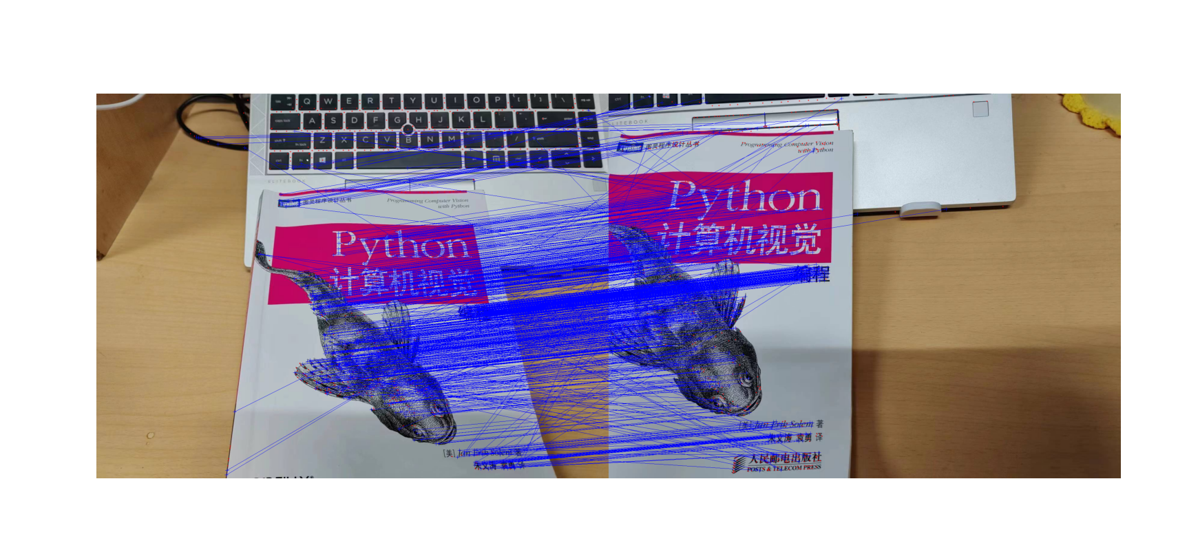
pic = draw_matches(img1, img2, keyarr_1, keyarr_2, matches)

plt.imshow(pic)
plt.axis('off')
plt.show()
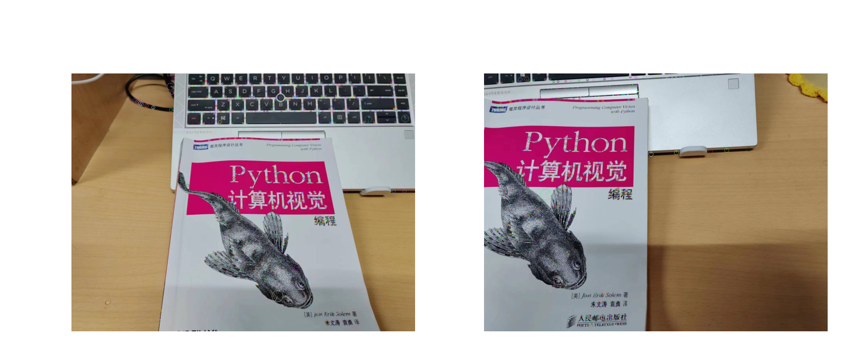

Harris角点检测与SIFT特征提取两者的区别
Harris角点检测算法是一个极为简单的角点检测算法。该算法的主要思想是,如果像素周围显示存在多于一个方向的边,我们认为该点为兴趣点。该点就称为角点
SIFT特征对于尺度,旋转和亮度都具有不变形,因此,它可以用于三维视角和噪声的可靠匹配。
3.实现匹配地理标记图像
python实现:
# -*- coding: utf-8 -*-

# from pylab import *
from pylab import *
from PIL import Image
from PCV.localdescriptors import sift
from PCV.tools import imtools
import pydot

# 将其设置为存储图像的路径
download_path = "F:\work\CV\ExmCode\ex2\graphimgset"
# 保存缩略图的路径(pydot需要完整的系统路径)
path = "F:\work\CV\ExmCode\ex2\graphimgset"

# 下载的文件名列表
imlist = imtools.get_imlist(download_path)
nbr_images = len(imlist)

# 提取特征
featlist = [imname[:-3] + 'sift' for imname in imlist]
for i, imname in enumerate(imlist):
    sift.process_image(imname, featlist[i])

matchscores = np.zeros((nbr_images, nbr_images))

for i in range(nbr_images):
    for j in range(i, nbr_images):  # 仅仅计算上三角
        print('comparing ', imlist[i], imlist[j])
        l1, d1 = sift.read_features_from_file(featlist[i])
        l2, d2 = sift.read_features_from_file(featlist[j])
        matches = sift.match_twosided(d1, d2)
        nbr_matches = sum(matches > 0)
        print('number of matches = ', nbr_matches)
        matchscores[i, j] = nbr_matches
print("The match scores is: \n", matchscores)

# 复制值
for i in range(nbr_images):
    for j in range(i + 1, nbr_images):  # 无需复制对角线
        matchscores[j, i] = matchscores[i, j]

# 可视化
threshold = 2  # 创建关联所需的最小匹配数目

g = pydot.Dot(graph_type='graph')  # 不使用默认的有向图

for i in range(nbr_images):
    for j in range(i + 1, nbr_images):
        if matchscores[i, j] > threshold:
            # 图像对中的第一幅图像
            im = Image.open(imlist[i])
            im.thumbnail((100, 100))
            filename = path + str(i) + '.png'
            im.save(filename)  # 需要大小合适的临时文件
            g.add_node(pydot.Node(str(i), fontcolor='transparent', shape='rectangle', image=filename))

            # 图像对中的第一幅图像
            im = Image.open(imlist[j])
            im.thumbnail((100, 100))
            filename = path + str(j) + '.png'
            im.save(filename)  # 需要大小合适的临时文件
            g.add_node(pydot.Node(str(j), fontcolor='transparent', shape='rectangle', image=filename))
            g.add_edge(pydot.Edge(str(i), str(j)))
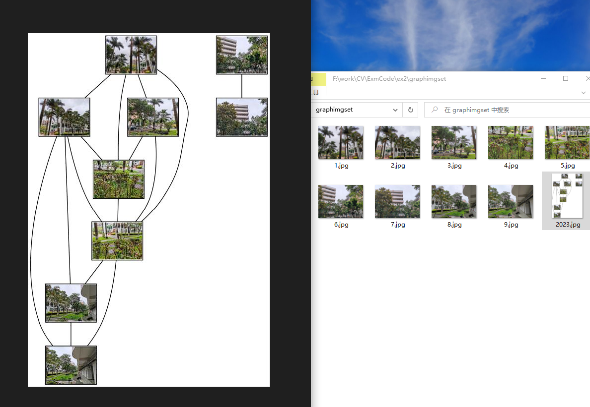
g.write_png('2023.png')
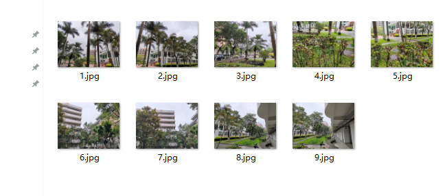
原始图像集
匹配完成图像缩略图:
更多推荐


 0
0 0
0- 0


 已为社区贡献1条内容

所有评论(0)