opencv Hough圆检测实现圆形表计在画面中位置的检测

行然梦实

1651人浏览 · 2024-12-16 22:51:22

行然梦实 · 2024-12-16 22:51:22 发布

前言

提醒：
文章内容为方便作者自己后日复习与查阅而进行的书写与发布，其中引用内容都会使用链接表明出处（如有侵权问题，请及时联系）。
其中内容多为一次书写，缺少检查与订正，如有问题或其他拓展及意见建议，欢迎评论区讨论交流。

文章目录

前言
代码与运行结果
Hough检测相关知识

代码与运行结果

opencv-python连接计算机摄像头，连接手机摄像头

import cv2
import numpy as np

# 初始化摄像头
cap = cv2.VideoCapture(0)

while True:
    # 读取视频流中的每一帧
    ret, frame = cap.read()
    if not ret:
        break

    # 获取图像的尺寸
    height, width = frame.shape[:2]
    center_x, center_y = width // 2, height // 2

    # 将图像转换为灰度图像
    gray = cv2.cvtColor(frame, cv2.COLOR_BGR2GRAY)

    # 应用高斯模糊，减少噪声
    blurred = cv2.GaussianBlur(gray, (15, 15), 0)

    # 使用霍夫圆变换检测圆形
    circles = cv2.HoughCircles(
        blurred, 
        cv2.HOUGH_GRADIENT, 
        dp=1.2, 
        minDist=900,  # 圆心之间的最小距离
        param1=30,  # 边缘检测的高阈值
        param2=70,  # 圆心检测的累加器阈值
        minRadius=1,  # 最小圆半径
        maxRadius=100  # 最大圆半径
    )

    # 如果检测到圆形
    if circles is not None:
        # 将圆的坐标转换为整数
        circles = np.round(circles[0, :]).astype("int")
        
        # 遍历所有检测到的圆形
        for (x, y, r) in circles:
            # 绘制圆心
            cv2.circle(frame, (x, y), 3, (0, 255, 0), -1)
            # 绘制圆形
            cv2.circle(frame, (x, y), r, (0, 255, 0), 3)
            
            # 判断圆心的方位
            if y < center_y - 50:
                vertical_position = "Top"
            elif y > center_y + 50:
                vertical_position = "Bottom"
            else:
                vertical_position = "Center"

            if x < center_x - 50:
                horizontal_position = "Left"
            elif x > center_x + 50:
                horizontal_position = "Right"
            else:
                horizontal_position = "Center"
            
            # 输出圆心的方位
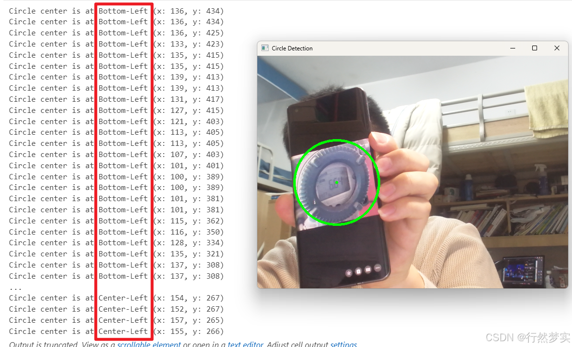
            print(f"Circle center is at {vertical_position}-{horizontal_position} (x: {x}, y: {y})")

    # 显示处理后的图像
    cv2.imshow("Circle Detection", frame)

    # 按下 'q' 键退出循环
    if cv2.waitKey(1) & 0xFF == ord('q'):
        break

# 释放摄像头资源
cap.release()
cv2.destroyAllWindows()

运行结果：

Hough直线检测数学原理

霍夫直线检测是一种在图像处理中用于检测直线的方法。其基本思想是将图像空间中的直线变换到参数空间中，通过在参数空间中寻找峰值来检测直线。
1. 直线的表示
在图像空间中，一条直线可以用以下公式表示：
$y = m x + b$
其中， $m$ 是斜率， $b$ 是截距。然而，当直线接近垂直时，斜率会变得非常大，导致数值不稳定。因此，霍夫变换使用极坐标形式来表示直线：
$\cos \theta + y \sin \theta$
其中， $r$ 是原点到直线的垂直距离， $\theta$ 是垂线与x轴的夹角。
2. 霍夫变换
霍夫变换的核心思想是将图像空间中的点映射到参数空间中。对于图像空间中的每一个点 $(x, y)$ ，我们可以在参数空间中绘制一条曲线，表示所有可能通过该点的直线。这条曲线可以表示为：
$\cos \theta + y \sin \theta$
通过改变 $\theta$ 的值（通常从0到180度），我们可以得到一系列的 $r$ 值。
3. 参数空间的积累
在参数空间中，每一条通过图像空间中点的曲线都会在某个点相交。这个交点代表了图像空间中的一条直线。因此，我们可以通过在参数空间中寻找交点来检测直线。
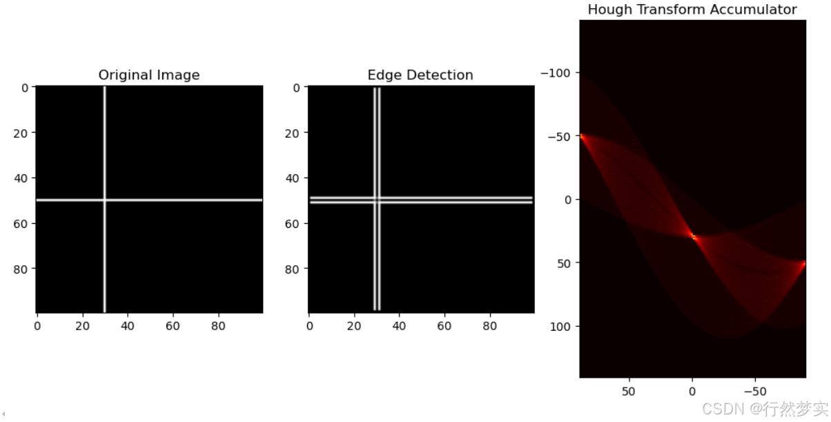
具体实现时，我们通常将参数空间离散化，形成一个累加器数组。对于图像空间中的每一个点，我们计算其在参数空间中对应的曲线，并在累加器数组中对应的位置加一。最终，累加器数组中的峰值位置就对应着图像空间中的直线。
4. 霍夫直线检测的步骤

边缘检测：首先对图像进行边缘检测，如使用Canny算子。
参数空间初始化：初始化一个累加器数组，用于存储参数空间中的值。
投票：对于边缘检测后的每一个点，计算其在参数空间中的对应曲线，并在累加器数组中投票。
检测峰值：在累加器数组中寻找峰值，这些峰值对应着图像空间中的直线。
5. 优点和缺点
优点：

能有效检测直线，即使直线存在断裂。
对噪声具有一定的鲁棒性。
缺点：
计算复杂度较高，特别是当图像尺寸较大时。
需要调整的参数较多，如累加器数组的大小、峰值的阈值等。
霍夫直线检测是一种强大的直线检测工具，在计算机视觉和图像处理领域有着广泛的应用。

手动实现代码

import numpy as np
import matplotlib.pyplot as plt

# 创建一个简单的合成图像
def create_sample_image():
    image = np.zeros((100, 100))
    # 添加几条直线
    for x in range(100):
        image[50, x] = 1  # 水平直线
        image[x, 30] = 1  # 垂直直线
    return image

# Sobel边缘检测
def sobel_edge_detection(image):
    Gx = np.array([[-1, 0, 1], [-2, 0, 2], [-1, 0, 1]])
    Gy = np.array([[-1, -2, -1], [0, 0, 0], [1, 2, 1]])
    edges = np.zeros_like(image)
    for i in range(1, image.shape[0] - 1):
        for j in range(1, image.shape[1] - 1):
            Sx = np.sum(Gx * image[i-1:i+2, j-1:j+2])
            Sy = np.sum(Gy * image[i-1:i+2, j-1:j+2])
            edges[i, j] = np.sqrt(Sx**2 + Sy**2)
    return edges

# 霍夫变换
def hough_transform(edges):
    thetas = np.deg2rad(np.arange(-90, 90))
    width, height = edges.shape
    diag_len = int(np.sqrt(width**2 + height**2))
    rhos = np.linspace(-diag_len, diag_len, diag_len * 2)
    accumulator = np.zeros((2 * diag_len, len(thetas)), dtype=np.uint64)

    for y in range(height):
        for x in range(width):
            if edges[y, x] > 0:
                for theta_idx in range(len(thetas)):
                    theta = thetas[theta_idx]
                    rho = x * np.cos(theta) + y * np.sin(theta)
                    rho_idx = int(rho + diag_len)
                    accumulator[rho_idx, theta_idx] += 1

    return accumulator, thetas, rhos

# 创建样本图像
sample_image = create_sample_image()

# 边缘检测
edges = sobel_edge_detection(sample_image)

# 霍夫变换
accumulator, thetas, rhos = hough_transform(edges)

# 显示结果
plt.figure(figsize=(12, 6))

plt.subplot(1, 3, 1)
plt.title('Original Image')
plt.imshow(sample_image, cmap='gray')

plt.subplot(1, 3, 2)
plt.title('Edge Detection')
plt.imshow(edges, cmap='gray')

plt.subplot(1, 3, 3)
plt.title('Hough Transform Accumulator')
plt.imshow(accumulator, cmap='hot', extent=[np.rad2deg(thetas[-1]), np.rad2deg(thetas[0]), rhos[-1], rhos[0]])

plt.show()

运行结果：

Hough圆检测数学原理

霍夫圆形检测是一种在图像中检测圆形物体的计算机视觉技术。它基于霍夫变换，这是一种用于检测图像中几何形状的算法。以下是霍夫圆形检测的详细原理和数学公式：

圆形的数学表示
一个圆形在二维图像空间中可以用其中心点 $x_0, y_0)$ 和半径 $r$ 来描述。其方程为：
$x - x_0)^2 + (y - y_0)^2 = r^2$
霍夫变换的基本思想
霍夫变换的基本思想是将图像空间中的点转换到参数空间中。在参数空间中，一个点对应于图像空间中的一个圆。通过在参数空间中寻找局部最大值，可以检测到图像中的圆形。
参数空间的构建
对于图像中的每个点 $(x, y)$ ，我们可以将其转换为参数空间中的一个圆。参数空间中的每个点 $x_0, y_0, r)$ 代表一个可能的圆心位置和半径。
累加器数组
霍夫圆形检测使用一个三维的累加器数组 $A(x_0, y_0, r)$ 来记录每个可能的圆心位置和半径的出现次数。初始时，累加器数组被设置为0。
投票过程
对于图像中的每个边缘点 $(x, y)$ ，我们遍历所有可能的半径 $r$ 和圆心角度 $\theta$ ，计算对应的圆心位置 $x_0, y_0)$ ，并在累加器数组中对应的位置增加1。计算公式为：
$x_0 = x - r \cos(\theta)$
$y_0 = y - r \sin(\theta)$
检测圆形
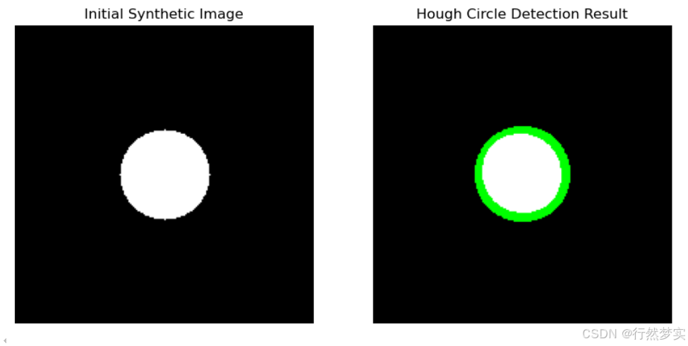
在投票过程完成后，累加器数组中的局部最大值对应于图像中的圆形。通过设定一个阈值，可以筛选出显著的圆形。
数学公式详细解释
7.1 圆的方程
圆的方程可以展开为：
$x^2 - 2xx_0 + x_0^2 + y^2 - 2yy_0 + y_0^2 = r^2$
7.2 参数空间的表示
在参数空间中，我们考虑所有可能的圆心 $x_0, y_0)$ 和半径 $r$ 。对于每个边缘点 $(x, y)$ ，我们将其转换为参数空间中的一系列点。
7.3 累加器数组的更新
对于每个边缘点 $(x, y)$ ，我们遍历所有可能的半径 $r$ ，并计算对应的圆心位置 $x_0, y_0)$ 。然后，我们在累加器数组 $A(x_0, y_0, r)$ 中对应的位置增加1：
$A(x_0, y_0, r) = A(x_0, y_0, r) + 1$
算法步骤
1. 预处理：对图像进行边缘检测，如使用Canny边缘检测器。
2. 初始化累加器数组：创建一个三维累加器数组 $A(x_0, y_0, r)$ ，并将所有值初始化为0。
3. 投票：对于每个边缘点 $(x, y)$ ，遍历所有可能的半径 $r$ ，计算对应的圆心位置 $x_0, y_0)$ ，并在累加器数组中对应的位置增加1。
4. 检测圆形：在累加器数组中寻找局部最大值，这些最大值对应于图像中的圆形。
注意事项

噪声敏感：霍夫圆形检测对噪声敏感，因此通常需要在检测前对图像进行预处理，如边缘检测、平滑等。
计算复杂度：由于需要遍历多个参数，霍夫圆形检测的计算复杂度较高，特别是当图像尺寸和半径范围较大时。

手动代码实现

import cv2
import numpy as np
import matplotlib.pyplot as plt

def generate_synthetic_image(size, circle_center, circle_radius):
    # 创建一个黑色背景的图像
    image = np.zeros((size, size), dtype=np.uint8)
    
    # 绘制一个白色圆形
    cv2.circle(image, circle_center, circle_radius, 255, -1)
    
    return image

def hough_circle_detection(image, edge_threshold, radius_range):
    # 边缘检测
    edges = cv2.Canny(image, 50, 150)

    # 初始化累加器
    height, width = image.shape
    accumulator = np.zeros((height, width, radius_range[1] - radius_range[0]))

    # 投票过程
    for y in range(height):
        for x in range(width):
            if edges[y, x] > edge_threshold:
                for r in range(radius_range[0], radius_range[1]):
                    for theta in range(0, 360):
                        a = x - r * np.cos(np.deg2rad(theta))
                        b = y - r * np.sin(np.deg2rad(theta))
                        if a >= 0 and a < width and b >= 0 and b < height:
                            accumulator[int(b), int(a), r - radius_range[0]] += 1

    # 检测圆形
    circles = []
    threshold = 0.5 * np.max(accumulator)
    for r in range(radius_range[1] - radius_range[0]):
        for y in range(height):
            for x in range(width):
                if accumulator[y, x, r] > threshold:
                    circles.append((x, y, r + radius_range[0]))

    return circles

# 生成合成图像
image_size = 200
circle_center = (100, 100)
circle_radius = 30
synthetic_image = generate_synthetic_image(image_size, circle_center, circle_radius)

# 设置参数
edge_threshold = 100
radius_range = (10, 50)  # 圆的半径范围

# 执行霍夫圆检测
detected_circles = hough_circle_detection(synthetic_image, edge_threshold, radius_range)

# 绘制检测结果
output_image = cv2.cvtColor(synthetic_image, cv2.COLOR_GRAY2BGR)
for x, y, r in detected_circles:
    cv2.circle(output_image, (x, y), r, (0, 255, 0), 2)

# 显示初始图像和检测结果
plt.figure(figsize=(10, 5))

plt.subplot(1, 2, 1)
plt.title('Initial Synthetic Image')
plt.imshow(synthetic_image, cmap='gray')
plt.axis('off')

plt.subplot(1, 2, 2)
plt.title('Hough Circle Detection Result')
plt.imshow(cv2.cvtColor(output_image, cv2.COLOR_BGR2RGB))
plt.axis('off')

plt.show()

运行结果：

乐奇 Rokid 开放社区

更多推荐

让界面替我“摇“一次：一个AR祈愿智能体的AIUI实践

乐奇 Rokid 开放社区

AR 智能眼镜并不是简单地在眼前放一块屏幕，而是把**摄像头、传感器、计算机视觉、空间定位、语音交互和云端服务**连接起来

乐奇 Rokid 开放社区

智能眼镜市场全景解析：从技术演进到产业格局

本文系统梳理智能眼镜市场，涵盖产品形态、技术演进、市场规模、产业链结构及竞争格局。指出智能眼镜正从音频交互向AR显示与空间计算演进，受AI大模型、供应链成熟与生态延伸驱动，呈现分层发展态势。虽面临场景刚需不足、续航重量矛盾与隐私挑战，但B端应用先行、AI原生设计与标准完善将推动行业迈向规模化渗透，未来需关注核心技术突破与真实使用数据。