方案

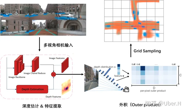
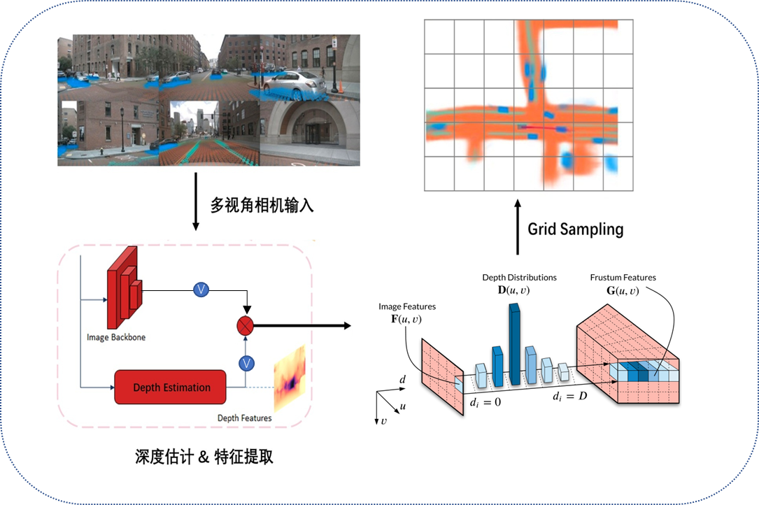
• 外积（Outer product）

这一步是LSS的最灵魂的操作。Depth distrbution(H,W,D) and image feature(H,W,C) combine to a frustum feature(H,W,D,C).

• Grid Sampling

这一步的目的就是将上面构造出的Frustum Feature 利用相机外参和内参转换到BEV视角下。具体过程是，通过限定好BEV视角的范围，划定好一个个的grid，将能够投影到相应grid 的 Feature 汇总到一个grid 里，之后再进行 "Splat"操作。这一步虽然听起来平平无奇，但是在具体的代码实现方面却有很多trick值得学习

BEVDepth 的LSS代码

首先看BEVDepth的LSS部分。代码中有一个BaseLSSFPN类，forward方法处理多帧图像，提取关键帧和过渡帧的BEV特征。在_forward_single_sweep方法里，首先提取图像特征，然后通过深度网络得到深度分布，再结合context特征。接着通过get_geometry生成视锥点云坐标，转换到BEV空间，最后用网格采样得到特征图。这里的关键步骤是深度预测、坐标变换和网格采样。

bevdepth/layers/backbones/base_lss_fpn.py

class BaseLSSFPN(nn.Module):
    def __init__(...):
        ...
    def forward(...):
        """
        Args:
            sweep_imgs:[1, 2, 6, 3, 256, 704],关键帧以及过渡帧图片
            mats_dict(dict):
                sensor2ego_mats:相机坐标系->车辆坐标系
                intrin_mats:相机内参
                ida_mats:图像数据增强矩阵
                sensor2sensor_mats:key frame camera to sweep frame camera,关键帧到过渡帧的变化矩阵
                bda_mat:bev特征增强矩阵    
        """
        # 提取关键帧的BEV特征 key_frame_res:[1, 80, 128, 128])
        key_frame_res = self._forward_single_sweep(...)
        
        for sweep_index in range(1, num_sweeps):
            #  提取过渡帧的bev特征
            feature_map = self._forward_single_sweep(...)
            ret_feature_list.append(feature_map)
        if is_return_depth:
            return torch.cat(ret_feature_list, 1), key_frame_res[1]
        return torch.cat(ret_feature_list, 1) 
        
    def _forward_single_sweep(...):
        # 提取环视图片特征
        # img_feats:[1, 1, 6, 512, 16, 44]
        img_feats = self.get_cam_feats(sweep_imgs)
        source_features = img_feats[:, 0, ...]
        
        # 提取Depth以及context
        depth_feature = self._forward_depth_net(...)
        # 预测的距离分布 depth:[6, 112, 16, 44]
        depth = depth_feature[:, :self.depth_channels].softmax(1)
        # 对应论文中的 Context Feature * Depth Distribution 操作
        img_feat_with_depth = ... # 
        
        # 车辆坐标系下的视锥坐标点 geom_xyz:[1, 6, 112, 16, 44, 3] 
        geom_xyz = self.get_geometry(...)
        # 将车辆坐标系的原点移动到左下角
        # 获得最终BEV特征 feature_map 
        geom_xyz = ((geom_xyz - (self.voxel_coord - self.voxel_size / 2.0)) /
                    self.voxel_size).int()
        
        if is_return_depth:
            # 训练时需要返回预测的深度，用lidar信号进行监督
            return feature_map.contiguous(), depth
        return feature_map.contiguous()
        
    def _forward_depth_net(...):
        return self.depth_net(feat, mats_dict)
    
    def get_geometry(...):
        """Transfer points from camera coord to ego coord
        Args:
            rots(Tensor): Rotation matrix from camera to ego.
            trans(Tensor): Translation matrix from camera to ego.
            intrins(Tensor): Intrinsic matrix.
            post_rots_ida(Tensor): Rotation matrix for ida.
            post_trans_ida(Tensor): Translation matrix for ida
            post_rot_bda(Tensor): Rotation matrix for bda.
        """
        # self.frustum:[112, 16, 44, 4] 视锥 
        # 在代码中的 get_geometry 方法中，使用了一个叫做 self.frustum 的变量，它的形状是 [112, 16, 44, 4]，代表了视锥中的空间点。
        # 视锥表示的是从相机视角出发，沿着视线方向一定距离范围内的区域，它是由相机内外参和图像增强矩阵等多个因素共同定义的。
        points = self.frustum
        
        #  乘以图像增强的逆矩阵
        points = ida_mat.inverse().matmul(points.unsqueeze(-1))
        
        # lamda * [x,y,1] = [lamda*x,lamda*y,lamda]
        # 像素坐标系转相机坐标系
        points = torch.cat(...)
        
        # cam_to_ego
        combine = sensor2ego_mat.matmul(torch.inverse(intrin_mat))
        points = combine.view(...)
        # 在 get_geometry 中的坐标变换后，生成的几何坐标（如 geom_xyz）可能会用作 GridSample 的采样网格，将这些坐标映射到新的特征图上。
        # 这样，你就能在目标坐标系（如自车坐标系或BEV）中获取经过变换后的特征。
        return points

地平线grid_sample 方法

地平线的grid_sample方法。他们的LSSTransformer分为生成深度特征、BEV坐标转换和生成视锥点云特征。生成深度特征后，他们将深度特征和图像特征分开进行BEV转换，以减少计算量。使用grid_sample进行特征采样，每个voxel采样多次（比如10次），然后将结果相加得到最终的BEV特征。这里的重点是多点采样和特征融合。

hat/models/task_modules/view_fusion/view_transformer.py

可将bev_lss的view_transformer分为3个部分：

• 生成深度特征
• 对深度特征和img_encoder_feature做bev坐标转换
• 生成视锥点云特征(frustum features)

接下来将对这三个部分做具体介绍的具体代码实现：

生成深度特征
生成depth为60的depth_feature，对depth_feature计算深度的score值。
对应代码:

self.depth_net = ConvModule2d(
    in_channels=in_channels,
    out_channels=depth,
    kernel_size=1,
    padding=0,
    stride=1,
    bias=False,
)

depth = self.softmax(self.depth_net(feats))

生成 bev_feature
为了减少mul计算量, 先把深度特征和 feature 分开做bev视角转换：

class LSSTransformer(ViewTransformer):
     ...
     def _spatial_transfom(self, feats, points):
        ...
        feat = feat.view(B, C, -1, W)
        dfeat = dfeat.view(B, 1, -1, H * W)
        homo_feats = []
        for i in range(self.num_points):
            homo_feat = self.grid_sample(
                feat, # [1,64,6*16,44]
                self.quant_stub(points[i]),
            ) #[1,64,128,128]
            homo_dfeat = self.dgrid_sample(
                dfeat,  #  [1,1,6*60,16*44]
                self.dquant_stub(points[i + self.num_points]),
            ) # [1,1,128,128]
            homo_feat = self.floatFs.mul(homo_feat, homo_dfeat)#视锥点云特征
            homo_feats.append(homo_feat)

其中，point的生成在_gen_reference_point，计算逻辑如下：
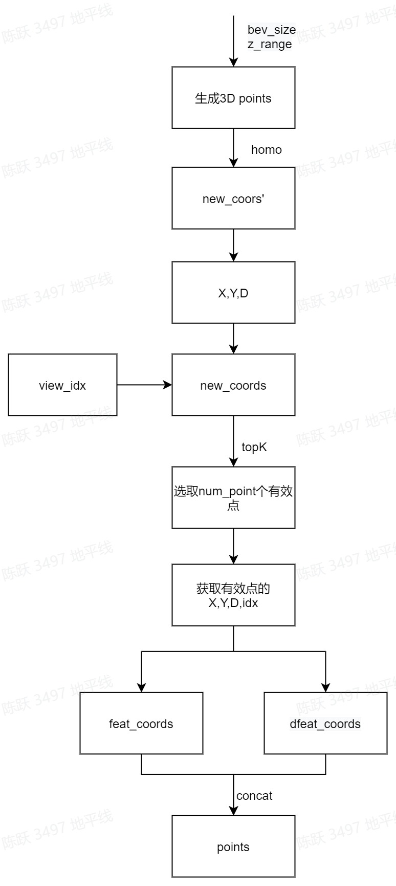生成点云特征

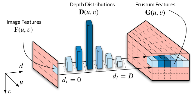
为了不遗失坐落在相同voxel中的点云特征，将对每个voxel都采样10次。

class LSSTransformer(ViewTransformer):
     ...
     def _spatial_transfom(self, feats, points):
        ...
        for i in range(self.num_points):
            homo_feat = self.grid_sample(
                feat,
                self.quant_stub(points[i]),
            )
            #num_points=10
            homo_dfeat = self.dgrid_sample(
                dfeat,
                self.dquant_stub(points[i + self.num_points]),
            )
            homo_feat = self.floatFs.mul(homo_feat, homo_dfeat)

最终将每个点云特征相加得到128x128x64的BEV特征图：

trans_feat = homo_feats[0]
for f in homo_feats[1:]:
    trans_feat = self.floatFs.add(trans_feat, f)

1. 为什么 Lss 的精度低于 IPM？

答：Lss 的输入分辨率是 256x704， 低于 IPM 的 512x960，所以精度更低。

2. Lss 输入的约束条件是什么？

答：Lss 在 grid_sample 前会做维度折叠，所以对 input_feature 的 h、w 有算子编译的约束条件， 目前为：H,W ∈ [1, 1024] 且 HW ≤ 7201024。

3. Lss 的 mul(depth,feature) 耗时大如何解决？

答：可以先通过 grid_sample 算子将 featuremap 的 H、W 转换为 [128,128] 后再做 mul 计算。

4. Lss 的 voxelpooling 如何实现？选取多少个点？

答：为了不遗失坐落在相同 voxel 中的点云特征，我们会对每个 voxel 采样 10 次， 并将每个点云特征相加得到 128x128x64 的 BEV 特征图，对应代码如下：

num_points=10
for i in range(self.num_points):    # 每个voxel采样10次
    homo_feat = self.grid_sample(
        feat,
        self.quant_stub(points[i]),
    )
    homo_dfeat = self.dgrid_sample(
        dfeat,
        self.dquant_stub(points[i + self.num_points]),
    )
    homo_feat = self.floatFs.mul(homo_feat, homo_dfeat)

trans_feat = homo_feats[0]
for f in homo_feats[1:]:
    trans_feat = self.floatFs.add(trans_feat, f)    # 点云特征相加

5. Lss 如何选择参考点？

答：point 的生成在 _gen_reference_point，会将 feature 范围外的无效点置为较大的值。 为了不取到无效点，会使用 topk（k=10，训练速度较快）将取值较小的前 10 个点进行集合。

6. Lss 如何处理 gridsample 输入较大的情况？

答：Lss 模型因为会在 gridsample 算子前将 3 个维度折叠为 1 个维度，因此其 HW 容易超出 7201024 的 BPU 算子约束限制。 此时建议在维度折叠（即 dfeat = dfeat.view(B, 1, -1, H * W)）前，先对可能超限的维度进行拆分，分别计算 gridsample，最后再将结果叠加。

对比

比较两者的流程。BEVDepth的流程可能更直接，深度预测和特征结合后，通过坐标变换到BEV，然后网格采样。而地平线的方法可能在网格采样前做了更多的优化，比如分解深度和特征的处理，多次采样后累加，以提高特征保留能力。

关键差异说明：

1. 采样机制：
   • BEVDepth：单次网格采样（geom_xyz.int()）
   • 地平线：多次网格采样（每个voxel采样10次后累加）
2. 特征处理：
   • BEVDepth：先融合特征与深度分布（Context*Depth）
   • 地平线：分离处理特征和深度（grid_sample分开执行）
3. 坐标生成：
   • BEVDepth：基于固定视锥生成几何坐标（self.frustum）
   • 地平线：动态生成多参考点（_gen_reference_point）
4. 计算优化：
   • 地平线：采用维度折叠（view(B,1,-1,H*W)）和量化策略（quant_stub）
   • BEVDepth：直接使用浮点坐标变换（sensor2ego_mat矩阵运算）

最终的网络模型onnx有区别

参考

https://yanyx.blog.csdn.net/article/details/138656353
https://developer.d-robotics.cc/forumDetail/143772473308124163