
脑机接口SSVEP经典算法 FBCCA滤波器组典型相关分析 matlab实战
Filter Bank Canonical Correlation Analysis (FBCCA) 是一种用于多通道脑电图(EEG)信号处理的算法,特别用于稳态视觉诱发电位(SSVEP)脑-机接口(BCI)系统中的信号分类。FBCCA结合了滤波器组(Filter Bank)和典型相关分析(Canonical Correlation Analysis, CCA)的技术,旨在提高不同频率刺激下SSVEP信号的分类性能。
项目地址:
项目首页 - FBCCA算法matlab实现:脑机接口SSVEP领域FBCCA算法的matlab实现代码。 - GitCode https://gitcode.com/foamz/FBCCA
目录
1.数据集使用
使用清华大学脑机接口团队的公开数据集,benchmark dataset。我下载了S1~S6。
数据集下载地址 清华大学脑机接口研究组
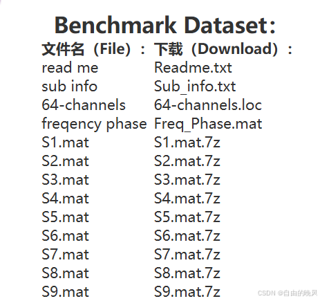
在FBCCA论文《Filter bank canonical correlation analysis for implementing a high-speed SSVEP-based brain–computer interface》中有提到
Nine electrodes over the parietal and occipital areas (Pz, PO5, PO3, POz, PO4, PO6, O1, Oz, and O2) were used to record SSVEPs. The electrode locations were selected toward high classification performance in a separate study using a 64-channel data set.
这段文字说明,只有位于顶叶和枕叶区域的9个电极区域信息,对SSVEP的分类性能是最好的。
然后根据64-channels.ioc文件,可以找出对应电极的数据存放在哪个通道,后续进行提取处理。
2.FBCCA运作流程
论文中这张图片大致描绘了整体运作流程。
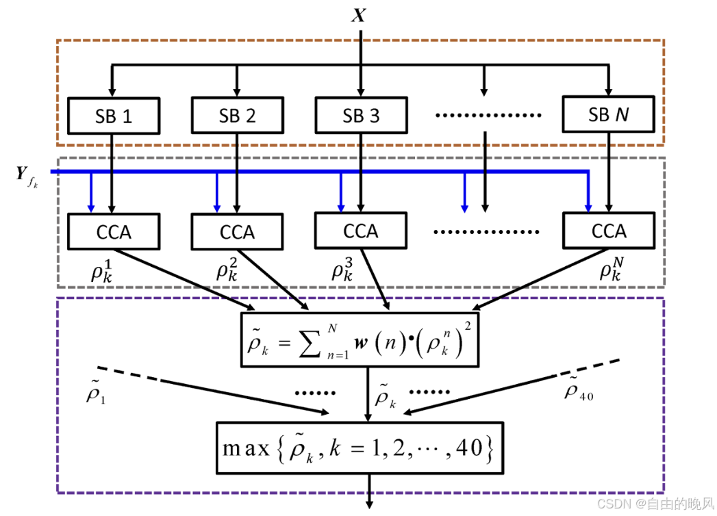
先将脑电信号送至滤波器组,在每个滤波器SB1、SB2、SB3......上并行滤波。对滤波数据分别进行CCA典型相关分析,然后将得到的相关系数的平方,分别乘以滤波器加权系数w(n),进行求和。得到一个滤波器组的 ~pk 。然后因为有40个刺激频率,所以理论上最终会有40个不同的相关系数组。找到每个相关系数组下最大的系数,其对应的频率即是SSVEP的频率。
关于w(n),其表达式为
w(n) = n^(-0.5) + 1.25
5个的话,w(n)=[1.2500 0.6704 0.5033 0.4268 0.3837]
关于滤波器组的设计,文章给出了M1、M2、M3三种滤波器组设计方法,对应下图的a,b,c。
对应方法的每个滤波器通带设计如下图红框所示,多个滤波器构成滤波器组。
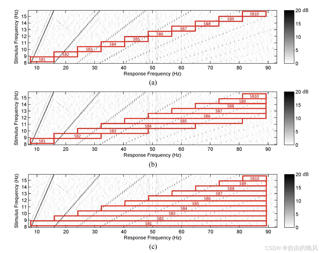
文章表示,按照M3样式设计的滤波器组,会使得该算法具有更高的性能。
To optimize the design of the filter bank, this study proposed and compared three methods:
- M1: sub-bands with equally spaced bandwidths;
- M2: sub-bands corresponding to individual harmonic frequency bands;
- M3: sub-bands covering multiple harmonic frequency bands.
The bandwidth of 80 Hz resulted in 10 sub-bands for these methods. Although all three methods covered the whole frequency band of 8-88 Hz, the results suggested that M3 can achieve the highest classification performance.
为了优化滤波器组的设计,本研究提出并比较了三种方法(M1:带宽相等的子带;M2:对应各个谐波频带的子带;M3:覆盖多个谐波频带的子带)。带宽为80 Hz的情况下,这三种方法得到的子带数量为10个。尽管这三种方法都覆盖了8-88 Hz的整个频率范围,结果表明M3可以获得最高的分类性能。
3.matlab实战
按照M3样式设计滤波器组,通带选择了5-90HZ。
(1) test_fbcca.m
测试主程序,其他文件都是函数。
% 1. 提取数据
% 定义文件名的前缀和后缀
file_prefix = 's';  % 文件名前缀
file_extension = '.mat';  % 文件扩展名
% 准确率验证信息
freq_list = zeros(1, 40);
fre_exam = load('Freq_Phase.mat');
% 2. 参数设置
sampling_rate = 250;  % 采样频率 250Hz
stim_freqs = [8, 9, 10, 11, 12, 13, 14, 15, ...
              8.2, 9.2, 10.2, 11.2, 12.2, 13.2, 14.2, 15.2, ...
              8.4, 9.4, 10.4, 11.4, 12.4, 13.4, 14.4, 15.4, ...
              8.6, 9.6, 10.6, 11.6, 12.6, 13.6, 14.6, 15.6, ...
              8.8, 9.8, 10.8, 11.8, 12.8, 13.8, 14.8, 15.8];  % 40个目标频率
t = 1:1000;

% 定义通带频率 wp 和阻带频率 ws
wp = {[5, 90], [14, 90], [22, 90], [30, 90], [38, 90]};  % 通带频率
ws = {[3, 92], [12, 92], [20, 92], [28, 92], [36, 92]};  % 阻带频率

% 采样率和滤波器阶数
srate = 250;
order = 15;
rp=0.5;
% 设计滤波器组
filterbank = generate_filterbank(wp, ws, srate, order, rp);  % 初始化滤波器组

% 滤波器权重系数
filterweights = arrayfun(@(idx_filter) (idx_filter + 1) ^ (-1.25) + 0.25, 0:4);

% 使用for循环读取每个文件
for h = 1:6
    % 构建文件名
    file_name = [file_prefix num2str(h) file_extension];

    % 检查文件是否存在
    if exist(file_name, 'file')
        % 加载文件
        data = load(file_name);
        eeg_data = data.data;  % 获取数据矩阵

        % 提取其中一个区块的数据
        for block_index = 1:size(eeg_data, 4)
            data_first_block = eeg_data(:, :, :, block_index);
            % 3. 处理数据
            for stim_index = 1:size(stim_freqs,2)
                % 提取目标刺激的数据,维度是 [64, 1500](64 个电极,1500 个时间点)
                data_at_time_point = data_first_block(:, :, stim_index);  % 去掉目标刺激维度,得到 [64, 1500]
                %提取顶叶和枕叶区域(Pz、PO5、PO3、POz、PO4、PO6、O1、Oz和O2)的ssvep信号
                data_at_time_point = data_at_time_point([48, 54, 55, 56, 57, 58, 61, 62, 63], :);
                % 提取当前刺激段的数据
                stim_data = data_at_time_point(:, 251:1250);  % 当前刺激段去除刺激前0.5s和刺激后0.5s  9*1000

                % 4. 带通滤波
                n_channels = size(stim_data, 1);  % 通道数,应该是 9
                n_samples = size(stim_data, 2);   % 每个通道的数据点数,应该是 1000

                % 初始化滤波后的信号
                Xs = zeros(length(filterbank), n_channels, n_samples);  % 每个滤波器的输出

                % 对每个滤波器进行滤波
                for i = 1:length(filterbank)  % 对每个滤波器
                    for c = 1:n_channels  % 对每个通道
                        % 使用 filtfilt 进行零相位滤波
                        Xs(i, c, :) = filtfilt(filterbank{i}, 1, stim_data(c, :));  % 每个通道的信号滤波
                    end
                    % 5. 使用FBCCA算法,将滤波后数据放入CCA
                    eeg_data_c =squeeze(Xs(i, :, :));
                    estimated_p = fbcca(eeg_data_c', sampling_rate, t,stim_freqs);
                    freq_list= freq_list+ filterweights(i) .* estimated_p;
                end
                [max_value, max_index] = max(freq_list);
                freq_list = zeros(1, 40);
                % 6. 输出当前刺激段的估计频率
                %fprintf('刺激段 %d 的估计频率是: %.2f Hz\n', stim_index, stim_freqs(max_index));
                fre_res(stim_index) = stim_freqs(max_index);
            end
            accuracy(block_index) = cplist(fre_res,fre_exam.freqs);
        end
        % 计算每个文件6个试次的平均准确率
        acc_list(h)=mean(accuracy);
    else
        disp(['文件 ' file_name ' 不存在']);
    end
    fprintf('S%d文件的准确率:%.2f%%\n', h, acc_list(h));
end
fprintf('6个文件总准确率:%.2f%%\n',mean(acc_list));
(2) generate_filterbank.m
用于生成滤波器组的函数
function filterbank = generate_filterbank(passbands, stopbands, srate, order, rp)
    if nargin < 4
        order = [];  % Set default for order if not provided
    end
    if nargin < 5
        rp = 0.5;  % Set default for rp if not provided
    end

    filterbank = {};  % Initialize the filterbank as a cell array
    % Loop through the passbands and stopbands
    for i = 1:length(passbands)
        wp = passbands{i};  % Passband
        ws = stopbands{i};  % Stopband

        % Normalize the frequencies by the Nyquist frequency (srate/2)
        wp_norm = wp / (srate / 2);
        ws_norm = ws / (srate / 2);

        if isempty(order)  % If order is not specified
            % Use cheb1ord to find the optimal order and cutoff frequencies
            [N, wn] = cheb1ord(wp_norm, ws_norm, 3, 40);  % Find order and normalized cutoff frequencies
            % Use cheby1 to design the filter with the calculated order
            sos = cheby1(N, rp, wn, 'bandpass', 's');  % Design the filter with 'sos'
        else
            % When order is specified, use the fixed order for the design
            sos = cheby1(order, rp, wp_norm, 'bandpass', 's');  % Design the filter with fixed order
        end

        filterbank{i} = sos;  % Append the filter to the filterbank
    end
end
(3) fbcca.m
FBCCA,使用的滤波器组主要在test_fbcca.m中设定,对数据滤波使用了。这里的文件fbcca,m其实还是cca,不过这里使用MATLAB内置函数canoncorr,来计算CCA。
% FBCCA算法
function [freq] = fbcca(eeg_data, fs, t,freq_list)
    % eeg_data: 输入的EEG数据,每个通道的信号 64*1000
    % fs: 采样频率
    % freq_list: 所有可能的刺激频率

    num_freqs = length(freq_list);
    num_channels = size(eeg_data, 1);
    C1_list = zeros(1, num_freqs); % 初始化存储 C1 的单元数组
   % n = 2:2:num_channels;
    for j = 1:num_freqs
        fre = freq_list(j);
        target_signal =[sin(2*pi*fre*t/fs);
                        cos(2*pi*fre*t/fs);
                        sin(4*pi*fre*t/fs);
                        cos(4*pi*fre*t/fs);
                        sin(6*pi*fre*t/fs);
                        cos(6*pi*fre*t/fs)]; % 6*1000
        target_signal = target_signal';  %1000*6
        [Wx, Wy, r] = canoncorr(eeg_data, target_signal);
        %r是典型相关系数
        [maxVals1, ~] = max(r);
        % 找到最大相关性的频率
        freq(j) = maxVals1^2;
    end
    %[maxval, index] = max(C1_list);
    %P = sqrt(max_value);  % 相关系数p等于λ,这里特征值是λ的平方,后面开根号
    %freq = maxval;
end
(4) cplist.m
将得到的频率数据与标定频率进行比较,得到准确率。
function accuracy = cplist(A, B)
    % compare_lists 函数:比较两个列表A和B的元素是否相同,并计算准确率
    % 输入:
    %   A - 第一个列表
    %   B - 第二个列表
    % 输出:
    %   accuracy - 两个列表元素相同的准确率(百分比)
    % 检查两个列表的长度是否相同
    if length(A) ~= length(B)
        error('列表A和B的长度不相同!');
    end
    % 比较A和B对应位置上的元素
    correct_count = sum(A == B);
    % 计算准确率
    accuracy = correct_count / length(A) * 100;
end
4.运行结果:
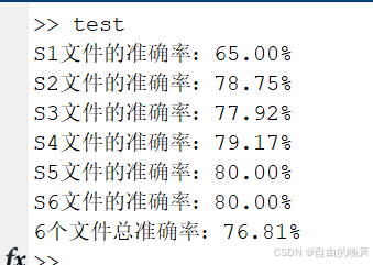
5.参考文献:
Xiaogang Chen, Yijun Wang, Shangkai Gao, Tzyy-Ping Jung and Xiaorong Gao,"Filter bank canonical correlation analysis for implementing a high-speed SSVEP-based brain–computer interface,"Journal of Neural Engineering, Volume 12, Number 4
更多推荐

 75
75 0
0- 0


 已为社区贡献1条内容

所有评论(0)