
数据结构(C语言)
目录
经典OJ算法题2:反转链表(思路:创建新链表或者利用三个指针)
经典OJ算法题7:返回倒数第k个节点(思路:快慢指针,快指针先走k步)
经典OJ算法题10:环形链表II(快慢指针+相遇点/相交链表)
经典OJ算法题11:随机链表的复制(原链表节点后插入新链表的复制节点)
一. 顺序表
1.1 顺序表的概念及结构
线性表
常见的线性表有顺序表、链表、栈、队列、字符串...,线性表在逻辑上是线性结构,也就是说是连续的一条直线。但是在物理结构上并不一定是连续的,线性表在物理上存储时,通常以数组和链式结构的形式存储。
1.2顺序表分类
静态顺序表
#define _CRT_SECURE_NO_WARNINGS
#include<stdio.h>

typedef int SLDataType;
#define N 7
typedef struct Seqlist
{
	SLDataType a[N];
	int szie;//顺序表当前的有效个数
}SL;
动态顺序表
#define _CRT_SECURE_NO_WARNINGS
#include<stdio.h>

typedef int SLDataType;

typedef struct Seqlist
{
	SLDataType* arr;
	int szie;//顺序表当前的有效个数
	int capacity;//空间大小
}SL;
1.3 顺序表的实现
在顺序表的实现中,我们用到了函数 exit(),我们便介绍一下:
void exit(int statue)exit 需要包含头文件 stdlib.h 来使用,它的主要作用是终止调用进程,参数 statue 是进程退出码,0 或者 EXIT_SUCCESS 表示正常退出;EXIT_FAILURE 或者 1 表示异常退出。
在 main 函数上 return 和 exit 的功能几乎一模一样,但在函数上想要终止调用进程,推荐用 exit。
顺序表的实现还会涉及扩容,这里提一嘴,扩容通常将原来的容量 *2。
#define _CRT_SECURE_NO_WARNINGS
#pragma once
typedef int SLDataType;

typedef struct Seqlist
{
	SLDataType* arr;
	int size;//顺序表当前的有效个数
	int capacity;//空间大小
}SL;

//顺序表初始化
void SLInit(SL* s);
//顺序表的销毁
void SLDestroy(SL* s);
//头部插入删除/尾部插入删除
void SLPushBack(SL* s, SLDataType x);
void SLPushFront(SL* s, SLDataType x);
void SLPopBack(SL* s);
void SLPopFront(SL* s);
//在指定位置插入/删除数据
void SLInsert(SL* ps, int pos, SLDataType x);
void SLErase(SL* ps, int pos);
//查找数据
int SLFind(SL* ps, SLDataType x);
//顺序表打印
void SLPrint(SL s);
#define _CRT_SECURE_NO_WARNINGS
#include"Seqlist.h"
#include<stdio.h>
#include<stdlib.h>
#include<assert.h>
//结构体初始化
void SLInit(SL* s)
{
s->arr = NULL;
s->size = 0;
s->capacity = 0;
}
//结构体销毁
void SLDestroy(SL* s)
{
if (s->arr)
{
free(s->arr);
}
s->arr = NULL;
s->capacity = s->size = 0;
}
void SLPushBack(SL* s, SLDataType x)
{
assert(s);
//温柔的解决方式
if (s == NULL)
{
return;
}
//插入前先看空间够不够
if (s->capacity == s->size)
{
//扩容
int newcapacity = s->capacity == 0 ? 4 : 2 * s->capacity;
SLDataType* tmp = (SLDataType*)realloc(s->arr, newcapacity * sizeof(SLDataType));
if (tmp == NULL)
{
perror("realloc");
exit(1);
}
//空间申请成功
s->arr = tmp;
s->capacity = newcapacity;
tmp = NULL;
}
s->arr[s->size++] = x;
}
void SLCheckCapacity(SL* s)
{
if (s->capacity == s->size)
{
int newcapacity = s->capacity == 0 ? 4 : 2 * s->capacity;
SLDataType* tmp = (SLDataType*)realloc(s->arr, newcapacity * sizeof(SLDataType));
if (tmp == NULL)
{
perror("realloc");
exit(1);
}
s->arr = tmp;
s->capacity = newcapacity;
tmp = NULL;
}
}
void SLPushFront(SL* s, SLDataType x)
{
assert(s);
SLCheckCapacity(&s);
for (int i = s->size - 1; i >= 0; i--)
{
s->arr[i + 1] = s->arr[i];
}
s->arr[0] = x;
s->size++;
}
void SLPopBack(SL* s)
{
assert(s);
assert(s->arr);
s->size--;
}
void SLPopFront(SL* s)
{
assert(s);
assert(s->arr);
for (int i = 0; i < s->size - 1; i++)
{
s->arr[i] = s->arr[i + 1];
}
s->size--;
}
void SLInsert(SL* ps, int pos, SLDataType x)
{
assert(ps && (pos <= ps->size && pos >= 0));
SLCheckCapacity(ps);
for (int i = ps->size - 1; i >= pos; i--)
{
ps->arr[i + 1] = ps->arr[i];
}
ps->arr[pos] = x;
ps->size++;
}
void SLErase(SL* ps, int pos)
{
assert(ps && ps->arr && (pos < ps->size && pos >= 0));
for (int i = pos; i < ps->size-1; i++)
{
ps->arr[i] = ps->arr[i + 1];
}
ps->size--;
}
int SLFind(SL* ps, SLDataType x)
{
assert(ps && ps->arr);
for (int i = 0; i < ps->size; i++)
{
if (ps->arr[i] == x)
return i;
}
return -1;
}
void SLPrint(SL s)
{
assert(s.arr);
for (int i = 0; i < s.size; i++)
{
printf("%d ", s.arr[i]);
}
printf("\n");
}1.5 顺序表经典算法
经典算法OJ题1:移除元素
int removeElement(int* nums, int numsSize, int val)
{
    int src=0;
    int dst=0;
    while(src<numsSize)
    {
      if(nums[src]==val)
      {
        src++;
      }
      else
      {
        nums[dst]=nums[src];
        dst++;
        src++;
      }
    }
    return dst;
}经典算法OJ题2:合并两个有序数组
void merge(int* nums1, int nums1Size, int m, int* nums2, int nums2Size, int n)
{
    int l1=m-1;
    int l2=n-1;
    int l3=m+n-1;
    while(l1>=0&&l2>=0)
   {
       if(nums1[l1]<=nums2[l2])
       {
           nums1[l3]=nums2[l2];
          l3--;
          l2--;
       }
      else
      {
          nums1[l3]=nums1[l1];
          l3--;
          l1--;
       }
   }
  while(l2>=0)
  {
    nums1[l3]=nums2[l2];
    l2--;
    l3--;
  }

}
1.6 顺序表的问题及思考
- 中间/头部的插入删除,时间复杂度为O(N)
- 增容需要申请新空间,拷贝数据,释放旧空间。会有不小的消耗。
- 增容一般是呈2倍的增长,势必会有一定的空间浪费。例如当前容量为100,满了以后增容到200,我们再继续插入了5个数据,后面没有数据插入了,那么就浪费了95个数据空间。
二. 链表
2.1 链表的概念及结构
链表是顺序表的一种,是一种物理存储结构上非连续、非顺序的存储结构,数据元素的逻辑顺序是通过链表中的指针链接次序实现的。
2.2 单链表的实现
#define _CRT_SECURE_NO_WARNINGS
#pragma once
typedef int SLDateType;
typedef struct SListNode
{
	SLDateType data;
	struct SListNode* next;
}SLTNode;
//遍历
void SLTPrint(SLTNode* phead);
//尾插/头插
void SLTPusnBack(SLTNode** phead, SLDateType x);
void SLTPusnFront(SLTNode** phead, SLDateType x);
//尾删/头删
void SLTPopBack(SLTNode** phead);
void SLTPopFront(SLTNode** phead);
//查找
SLTNode* SLTFind(SLTNode* phead, SLDateType x);
//在指定位置之前插入数据
void SLTInsert(SLTNode** phead, SLTNode* pos, SLDateType x);
//在指定位置之后插入数据
void SLTInserAfter(SLTNode* pos, SLDateType x);
//删除pos的节点
void SLTErease(SLTNode** phead, SLTNode* pos);
//删除pos之后的节点
void SLTEreaseAfter(SLTNode* pos);
//销毁链表
void SListDestroy(SLTNode** phead);
#define _CRT_SECURE_NO_WARNINGS
#include"Slist.h"
#include<assert.h>
#include<stdlib.h>
#include<stdio.h>

void SLTPrint(SLTNode* phead)
{
	SLTNode* pcur = phead;
	while (pcur)
	{
		printf("%d->", pcur->data);
		pcur = pcur->next;
	}
	printf("NULL\n");
}

SLTNode* SLTBuyNode(SLDateType x)
{
	SLTNode* newcode = (SLTNode*)malloc(sizeof(SLTNode));
	if (newcode == NULL)
	{
		perror("malloc");
		exit(EXIT_FAILURE);
	}
	newcode->data = x;
	newcode->next = NULL;
	return newcode;
}

void SLTPusnBack(SLTNode** phead, SLDateType x)
{
	assert(phead);
	SLTNode* newcode = SLTBuyNode(x);
	if (*phead == NULL)
	{
		*phead = newcode;
		return;
	}
	SLTNode* ptail = *phead;
	while (ptail->next)
	{
		ptail = ptail->next;
	}
	ptail->next = newcode;
}

void SLTPusnFront(SLTNode** phead, SLDateType x)
{
	assert(phead);
	SLTNode* newcode = SLTBuyNode(x);
	newcode->next = *phead;
	*phead = newcode;
}

void SLTPopBack(SLTNode** phead)
{
	assert(*phead && phead);
	if ((*phead)->next == NULL)
	{
		free(*phead);
		*phead = NULL;
		return;
	}
	SLTNode* ptail = *phead;
	while (ptail->next->next)
	{
		ptail = ptail->next;
	}
	free(ptail->next);
	ptail->next = NULL;
}

void SLTPopFront(SLTNode** phead)
{
	assert(phead && *phead);
	SLTNode* next = *phead;
	*phead = (*phead)->next;
	free(next);
}

SLTNode* SLTFind(SLTNode* phead, SLDateType x)
{
	assert(phead);
	SLTNode* pcur = phead;
	while (pcur)
	{
		if (pcur->data == x)
		{
			return pcur;
		}
		pcur = pcur->next;
	}
	return NULL;
}

void SLTInsert(SLTNode** phead, SLTNode* pos, SLDateType x)
{
	assert(phead && *phead);
	assert(pos);
	SLTNode* newnode = SLTBuyNode(x);
	SLTNode* cur = *phead;
	if (*phead == pos)
	{
		newnode->next = *phead;
		*phead = newnode;
		return;
	}
	while (cur->next)
	{
		if (cur->next == pos)
		{
			newnode->next = cur->next;
			cur->next = newnode;
			break;
		}
		cur = cur->next;
	}
}

void SLTInserAfter(SLTNode* pos, SLDateType x)
{
	assert(pos);
	SLTNode* newnode = SLTBuyNode(x);
	newnode->next = pos->next;
	pos->next = newnode;
}

void SLTErease(SLTNode** phead, SLTNode* pos)
{
	assert(phead && *phead);
	assert(pos);
	SLTNode* cur = *phead;
	if (cur == pos)
	{
		*phead = cur->next;
		free(cur);
		return;
	}
	while (cur->next)
	{
		if (cur->next == pos)
		{
			cur->next = pos->next;
			free(pos);
			pos = NULL;
			break;
		}
		cur = cur->next;
	}
}

void SLTEreaseAfter(SLTNode* pos)
{
	assert(pos && pos->next);
	SLTNode* cur = pos->next;
	pos->next = pos->next->next;
	free(cur);
	cur = NULL;
}

void SListDestroy(SLTNode** phead)
{
	assert(phead && *phead);
	SLTNode* pcur = *phead;
	while (pcur)
	{
		SLTNode* next = pcur->next;
		free(pcur);
		pcur = next;
	}
	*phead = NULL;
}
2.3 链表的分类
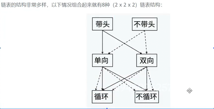
这里我们提一嘴我们会学的单链表和双向链表,单链表严格来讲是不带头、单向、不循环的链表,而双向链表是带头、双向、循环的链表。
这里说的带头不带头,不是我们平常认为的第一个有效节点,而是带有哨兵位的链表,哨兵位不存储数据,只用来占位。
2.4 链表经典算法
经典OJ算法题1:移除链表元素(思路:创建新链表)
经典OJ算法题2:反转链表(思路:创建新链表或者利用三个指针)
经典OJ算法题3:链表的中间节点 (思路:快慢指针)
经典OJ算法题4:合并两个有序链表
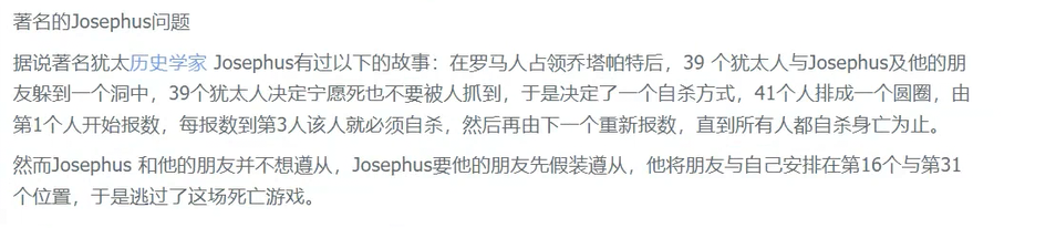
经典OJ算法题5:环形链表的的约瑟夫问题
经典OJ算法题6:分割链表
经典OJ算法题7:返回倒数第k个节点(思路:快慢指针,快指针先走k步)
经典OJ算法题8:链表的回文结构(查找中间节点+逆置)
经典OJ算法题8:相交链表(判断是否相交并返回指针)
经典OJ算法题9:环形链表(快慢指针)
关于算法题9,我们还衍生出几个问题:
1.为什么一定会相遇,有没有可能会错过?假设slow进环时,fast跟slow距离是N,每次追击二者之间的距离都会减一,那么第N次追击时,二者距离变为0。
2.slow 一次走1步,fast 走3步,4步,n步呢?
我们以 fast 走3步为例,N时偶数时,第一轮就追上;N是奇数,第一轮追不上,距离变成C-1(C是环的长度),如果C-1是偶数,下一轮就追上了;如果C-1是奇数,那么就永远追不上。
3.是否真的追不上?
我们以第二问的 fast 走3步为例,假设当 slow 进环时,slow 走过的路程是L,那么 fast 走过的路程是 L+x*C+C-N(x表示绕圈的次数),两个等式之间的关系是3L=L+x*C+C-N
=> 2L=x*C+C-N。当N是奇数,C是偶数时,等式:偶数=x*偶数+偶数-奇数。(这里我们提一嘴,偶数乘以任何数都是偶数,而偶数±奇数为奇数),我们可以发现这个情况是不存在的。
经典OJ算法题10:环形链表II(快慢指针+相遇点/相交链表)
这里说说为什么一个指针从头节点开始走,另一个指针从相遇点开始走,二者相遇的节点就是环开始的节点:
当slow走1步,fast走2步时,我们不妨来看看相遇时二者的路程,slow走了L+N(L表示在到达环开始的节点的路程,N表示相遇时slow在环上的路程),fast走了L+x*Q+N(Q是整个环的路程,Q是一定>N的,因为当slow走进环时,slow与fast的最远距离是Q-1,此后每追击一次,二者距离-1,那么slow最多走Q-1就被追上),可列等式2*(L+N)=L+x*Q+N =>
L+N=x*Q => L=(x-1)*Q+Q-N。
经典OJ算法题11:随机链表的复制(原链表节点后插入新链表的复制节点)
2.5 双向链表
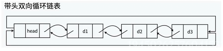
双向链表的结构
双向链表的实现
#define _CRT_SECURE_NO_WARNINGS
#include<stdlib.h>
typedef int LTDataType;

typedef struct ListNode
{
    LTDataType x;
    struct ListNode* next;
    struct ListNode* prev;
}ListNode;
//销毁
void LTDestroy(ListNode* phead);
//打印
void LTPrint(ListNode* phead);
//初始化
void LTInit(ListNode** phead);
//尾插
void LTPushBack(ListNode* phead, LTDataType x);
//头插
void LTPushFront(ListNode* phead, LTDataType x);
//尾删
void LTPopBack(ListNode* phead);
//头删
void LTPopFront(ListNode* phead);
//查找数据
ListNode* LTFind(ListNode* phead, LTDataType x);
//在pos位置之后插入数据
void LTInsert(ListNode* pos, LTDataType x);
//删除pos节点
void LTErase(ListNode* pos);
#define _CRT_SECURE_NO_WARNINGS
#include"Slist2.h"
#include<stdio.h>
#include<assert.h>
ListNode* LTBuyNode(LTDataType x)
{
ListNode* newnode = (ListNode*)malloc(sizeof(ListNode));
if (newnode == NULL)
{
perror("malloc");
exit(EXIT_FAILURE);
}
newnode->x = x;
newnode->next = newnode;
newnode->prev = newnode;
return newnode;
}
void LTInit(ListNode** phead)
{
*phead = LTBuyNode(-1);
}
void LTPushBack(ListNode* phead, LTDataType x)
{
assert(phead);
ListNode* newnode = LTBuyNode(x);
newnode->prev = phead->prev;
newnode->next = phead;
phead->prev->next = newnode;
phead->prev = newnode;
}
void LTPushFront(ListNode* phead, LTDataType x)
{
assert(phead);
ListNode* newnode = LTBuyNode(x);
newnode->next = phead->next;
newnode->prev = phead;
phead->next->prev = newnode;
phead->next = newnode;
}
void LTPrint(ListNode* phead)
{
assert(phead);
ListNode* cur = phead->next;
while (cur != phead)
{
printf("%d->", cur->x);
cur = cur->next;
}
printf("\n");
}
void LTPopBack(ListNode* phead)
{
assert(phead && phead->next != phead);
ListNode* cur = phead->prev;
phead->prev = cur->prev;
cur->prev->next = phead;
free(cur);
cur = NULL;
}
void LTPopFront(ListNode* phead)
{
assert(phead && phead->next != phead);
ListNode* cur = phead->next;
phead->next = cur->next;
cur->next->prev = phead;
free(cur);
cur = NULL;
}
ListNode* LTFind(ListNode* phead, LTDataType x)
{
assert(phead && phead->next != NULL);
ListNode* cur = phead->next;
while (cur != phead)
{
if (cur->x == x)
{
return cur;
}
cur = cur->next;
}
return NULL;
}
void LTInsert(ListNode* pos, LTDataType x)
{
assert(pos);
ListNode* newnode = LTBuyNode(x);
pos->next->prev = newnode;
newnode->next = pos->next;
pos->next = newnode;
newnode->prev = pos;
}
void LTErase(ListNode* pos)
{
assert(pos);
pos->prev->next = pos->next;
pos->next->prev = pos->prev;
free(pos);
pos = NULL;
}
void LTDestroy(ListNode* phead)
{
assert(phead);
ListNode* cur = phead->next;
while (cur != phead)
{
ListNode* next = cur->next;
free(cur);
cur = next;
}
free(phead);
phead = NULL;
}LTErase 和 LTDestroy 参数理论上要传二级,因为我们要求让形参的改变影响到实参,但是为了保持接口的一致性才传的一级。
传一级存在的问题是,当形参 phead 置为 NULL 后,实参 node 不会被修改为 NULL,因此解决办法是:调用完方法后手动将实参置为 NULL。
三. 算法的时间复杂度和空间复杂度
3.1 时间复杂度的概念
在计算机科学中,算法的时间复杂度是一个函数,它定量描述了该算法的运行时间。一个算法执行所耗费的时间,从理论上说,是不能算出来的,只有你把你的程序放在机器上跑起来,才能知道。但是我们需要每个算法都上机测试吗?是可以都上机测试,但是这很麻烦,所以才有了时间复杂度这个分析方式。一个算法所花费的时间与其中语句的执行次数成正比例,算法中的基本操作的执行次数,为算法的时间复杂度。
即:找到某条基本语句与问题规模N之间的数学表达式,就是算出了该算法的时间复杂度。
3.2 大O的渐进表示法
我们一般用大O渐进表示法来计算复杂度。
大O符号(Big O notation):是用于描述函数渐进行为的数学符号。
推导大O阶方法:
- 用常数1取代运行时间中的所有加法常数。
- 在修改后的运行次数函数中,只保留最高阶项。
- 如果最高阶项存在且不是1,则去除与这个项目相乘的常数。得到的结果就是大O阶。
另外有些算法的时间复杂度存在最好、平均和最坏情况:
- 最坏情况:任意输入规模的最大运行次数(上界)
- 平均情况:任意输入规模的期望运行次数
- 最好情况:任意输入规模的最小运行次数(下界)
例如:在一个长度为N数组中搜索一个数据x
- 最好情况:1次找到
- 最坏情况:N次找到
- 平均情况:N/2次找到
在实际中一般情况关注的是算法的最坏运行情况,所以数组中搜索数据时间复杂度为O(N)
3.3 复杂度的OJ练习
经典OJ算法题1:消失的数字(利用异或)
经典OJ算法题2:轮转数组(三个逆置)
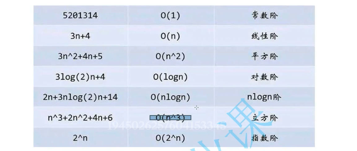
3.4 常见的复杂度对比
3.5 空间复杂度
- 空间复杂度也是一个数学表达式,是对一个算法在运行过程中临时占用存储空间大小的量度。
- 空间复杂度不是程序占用了多少bytes的空间,因为这个也没太大意义,所以空间复杂度算的是变量的个数。
- 空间复杂度计算规则基本跟实践复杂度类似,也使用大O渐进表示法。
- 注意:函数运行时所需要的栈空间(存储参数、局部变量、一些寄存器信息等)在编译期间已经确定好了,因此空间复杂度主要通过函数在运行时显式申请的额外空间来确定。
常见的空间复杂度有三个: O(1) O(N) O(N^2)
实例1:
//计算这个的空间复杂度
void BubbleSort(int* a, int n)
{
    assert(a);
    for (size_t end = n; end > 0; --end)
    {
        int exchange = 0;
        for (size_t i = 1; i < end; ++i)
        {
            if (a[i-1] > a[i])
            {
                Swap(&a[i-1], &a[i]);
                exchange = 1;
            }
        }

        if (exchange == 0)
            break;
    }
}
我们可以看到有变量 end、exchange、i,l量级是常数级别,那么空间复杂度是O(1)。为什么不算n 和 a 呢?这是因为计算空间复杂度时只算算法内部新开辟的临时空间。
实例2:
void _rotate(int* nums, int numsSize, int k, int* tmp)
{
    k %= numsSize;
    int n = numsSize;

    memcpy(tmp, nums + n - k, sizeof(int) * k);
    memcpy(tmp + k, nums, sizeof(int) * (n - k));
    memcpy(nums, tmp, sizeof(int) * (n));
}

void rotate(int* nums, int numsSize, int k) {
    int tmp[numsSize];
    _rotate(nums, numsSize, k, tmp);
}
在经典OJ算法题2中,如果想不到三次逆置,我们也可以考虑另开辟一个数组,用memcpy进行三次复制。那么这个的空间复杂度是多少呢?首先需要计算的变量有tmp、n,但是 tmp 是线性阶,我们就不在考虑 n ,那么这个的空间复杂度是O(n)。
实例3:
//计算这个的空间复杂度
long long Fac(size_t N)
{
    if(N == 0)
        return 1;
    return Fac(N - 1) * N;
}
每一次递归都会调用 Fac(N-1) ,递归的深度是 N-1,且每一层栈帧的空间是常数级别 O(1),所以总的空间复杂度是O(N)。
四. 栈
4.1 栈的概念及结构
栈:一种特殊的线性表,其只允许在固定的一端进行插入和删除元素操作。进行数据插入和删除操作的一端称为栈顶,另一端称为栈底。栈中的数据元素遵守后进先出LIFO(Last In First Out)的原则。
压栈:栈的插入操作叫做进栈/压栈/入栈,入数据在栈顶。
出栈:栈的删除操作做出栈。出数据也在栈顶。
4.2 栈的实现
#define _CRT_SECURE_NO_WARNINGS
#include<stdbool.h>
#pragma once
typedef int StackDateType;
typedef struct Stack
{
	StackDateType* arr;
	int capacity;
	int top;
}ST;

void STInit(ST* pst);
void STDestroy(ST* pst);
void STPush(ST* pst,StackDateType x);
void STPop(ST* pst);
StackDateType STTop(ST* pst);
bool STEmpty(ST* pst);
int STSize(ST* pst);
#define _CRT_SECURE_NO_WARNINGS
#include<stdio.h>
#include<stdlib.h>
#include"Stack.h"
#include<assert.h>
void STInit(ST* pst)
{
assert(pst);
pst->arr = NULL;
pst->capacity = 0;
pst->top = 0;
}
void STDestroy(ST* pst)
{
assert(pst);
free(pst->arr);
pst->arr = NULL;
pst->capacity = 0;
pst->top = 0;
}
void STPush(ST* pst, StackDateType x)
{
//断言是否为空
assert(pst);
//扩容
if (pst->top == pst->capacity)
{
int newcapacity = pst->capacity ? 2 * pst->capacity : 4;
StackDateType* tmp = (StackDateType*)realloc(pst->arr, newcapacity * sizeof(StackDateType));
if (tmp == NULL)
{
perror("realloc");
exit(EXIT_FAILURE);
}
pst->arr = tmp;
pst->capacity = newcapacity;
tmp = NULL;
}
//插入数据
pst->arr[pst->top] = x;
pst->top++;
}
void STPop(ST* pst)
{
assert(pst);
assert(pst->top > 0);
pst->top--;
}
StackDateType STTop(ST* pst)
{
assert(pst);
assert(pst->top > 0);
return pst->arr[pst->top - 1];
}
bool STEmpty(ST* pst)
{
assert(pst);
return pst->top == 0;
}
int STSize(ST* pst)
{
assert(pst);
return pst->top;
}五. 队列
5.1 队列的概念及结构
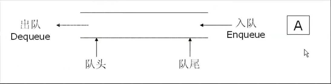
队列:只允许在一端进行插入数据操作,在另一端进行删除数据操作的特殊线性表,队列具有先进先出FIFO(First In First Out) 入队列:进行插入操作的一端称为队尾 出队列:进行删除操作的一端称为队头
5.2 队列的实现
#define _CRT_SECURE_NO_WARNINGS
#include<stdbool.h>

typedef int QDateytpe;

typedef struct QueueNode
{
	QDateytpe x;
	struct QueueNode* next;
}QNode;

typedef struct Queue
{
	QNode* phead;
	QNode* ptail;
	int size;
}Queue;

//初始化
void QueueInit(Queue* pq);
//销毁
void QueueDestroy(Queue* pq);
//插入
void QueuePush(Queue* pq,QDateytpe x);
//删除
void QueuePop(Queue* pq);
//大小
int QueueSize(Queue* pq);
//提取队首
QDateytpe QueueFront(Queue* pq);
//提取队尾
QDateytpe QueueBack(Queue* pq);
//判空
bool QueueEmpty(Queue* pq);
#define _CRT_SECURE_NO_WARNINGS
#include"Queue.h"
#include<stdlib.h>
#include<assert.h>
void QueueInit(Queue* pq)
{
assert(pq);
pq->phead = NULL;
pq->ptail = NULL;
pq->size = 0;
}
void QueueDestroy(Queue* pq)
{
assert(pq);
QNode* pcur = pq->phead;
while (pcur)
{
QNode* next = pcur->next;
free(pcur);
pcur = next;
}
pq->phead = pq->ptail = NULL;
pq->size = 0;
}
void QueuePush(Queue* pq, QDateytpe n)
{
QNode* newnode = (QNode*)malloc(sizeof(QNode));
if (newnode == NULL)
{
perror("malloc");
exit(EXIT_FAILURE);
}
newnode->next = NULL;
newnode->x = n;
if (pq->ptail == NULL)
{
pq->phead = newnode;
pq->ptail = newnode;
}
else
{
pq->ptail->next = newnode;
pq->ptail = newnode;
}
pq->size++;
}
void QueuePop(Queue* pq)
{
assert(pq && pq->phead);
if (pq->phead==pq->ptail)
{
free(pq->ptail);
pq->phead = pq->ptail = NULL;
}
else
{
QNode* pop = pq->phead;
pq->phead = pq->phead->next;
free(pop);
}
pq->size--;
}
QDateytpe QueueFront(Queue* pq)
{
assert(pq && pq->phead);
return pq->phead->x;
}
QDateytpe QueueBack(Queue* pq)
{
assert(pq && pq->phead);
return pq->ptail->x;
}
int QueueSize(Queue* pq)
{
assert(pq);
return pq->size;
}
bool QueueEmpty(Queue* pq)
{
assert(pq);
return pq->size == 0;
}5.3 栈和队列的面试题
经典OJ算法题1:用队列实现栈
经典OJ算法题2:设计循环队列
经典OJ算法题3:用栈实现队列
六. 树
6.1 树的概念及结构
6.1.1 树的概念
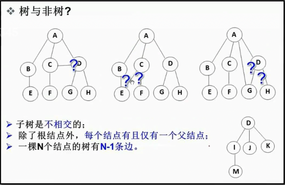
树是一种非线性的数据结构,它是由 n(n>=0)个有限结点组成一个具有层次关系的集合。把它叫做树是因为它看起来像一棵倒挂的树,也就是说它是根朝上,而叶朝下的。
- 有一个特殊的结点,称为根结点,根结点没有前驱结点
- 除根结点外,其余结点被分成 M (M>0) 个互不相交的集合 T1、T2、……、Tm,其中每一个集合 Ti (1<= i <= m) 又是一棵结构与树类似的子树。每棵子树的根结点有且只有一个前驱,可以有 0 个或多个后继。
- 因此,树是递归定义的。
6.1.2 树的基本概念
- 节点的度:一个节点含有的子树的个数称为该节点的度
- 叶节点或终端节点:度为 0 的节点称为叶节点
- 非终端节点或分支节点:度不为 0 的节点
- 双亲节点或父节点:若一个节点含有子节点,则这个节点称为其子节点的父节点
- 孩子节点或子节点:一个节点含有的子节点的根节点称为该节点的子节点
- 兄弟节点:具有相同父节点的节点互称为兄弟节点
- 树的度:一棵树中,最大的节点的度称为树的度
- 节点的层次:从根开始定义起,根为第 1 层,根的子节点为第 2 层,以此类推
- 树的高度或深度:树中节点的最大层次
- 堂兄弟节点:双亲在同一层的节点互为堂兄弟
- 节点的祖先:从根到该节点所经分支上的所有节点
- 子孙:以某节点为根的子树中任一节点都称为该节点的子孙
- 森林:由 m(m>0)棵互不相交的树的集合称为森林
6.2 二叉树概念及结构
6.2.1 概念
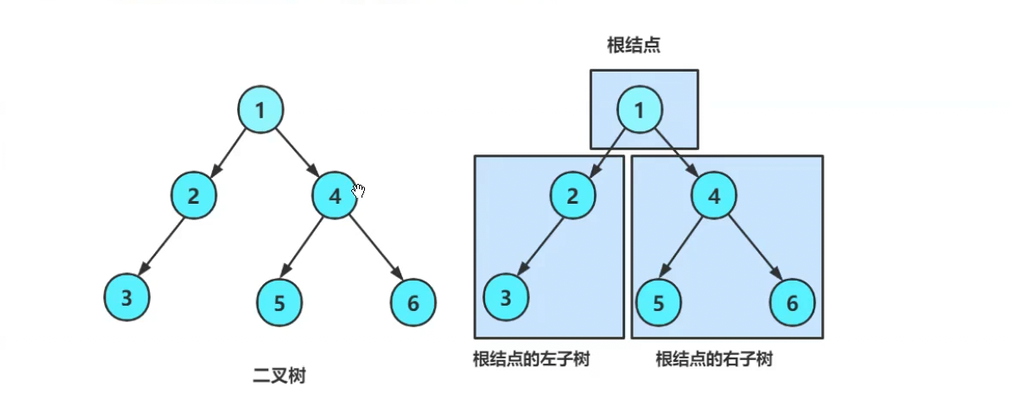
一棵二叉树是结点的一个有限集合,该集合:
- 或者为空
- 由一个根节点加上两棵别称为左子树和右子树的二叉树组成
从上面可以看出:
- 二叉树不存在度大于2的节点
- 二叉树的子树有左右之分,次序不能颠倒,因此二叉树是有序树
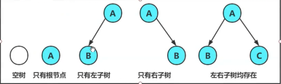
注意:对于任何二叉树都是由以下几种情况复合而成的:
6.2.2 特殊的二叉树
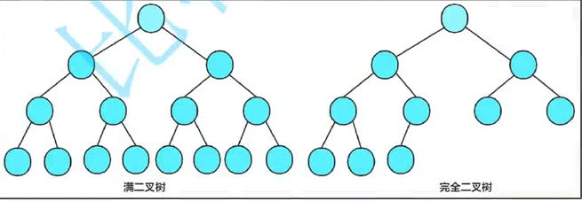
满二叉树:一个二叉树,如果每一个层的结点数都达到最大值,则这个二叉树就是满二叉树。也就是说,如果一个二叉树的层数为 K,且结点总数是2^k−1,则它就是满二叉树。
完全二叉树:完全二叉树是效率很高的数据结构,完全二叉树是由满二叉树而引出来的。对于深度为 K 的,有 n 个结点的二叉树,当且仅当其每一个结点都与深度为 K 的满二叉树中编号从 1 至 n 的结点一一对应时称之为完全二叉树。 要注意的是满二叉树是一种特殊的完全二叉树。
6.2.3 二叉树的存储
顺序存储
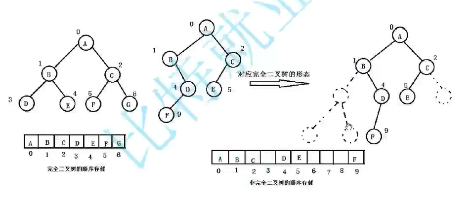
完全二叉树采用顺序存储有一个好处,可以通过父节点(子节点)帮助我们快速找到对应的子节点(父节点):假设父亲在数组的下标是 j,那么它的左孩子在数组的下标是 2*j+1,右孩子在数组的下标是 2*j+2;同理假设一个孩子在数组的下标是 i,如果 i 是奇数,那它是左孩子,它的父亲在数组的下标是(i - 1)/ 2;i 是偶数,那他是右孩子,他的父亲在数组的下标是(i - 2)/ 2。
非完全二叉树也可以采用顺序存储,但是不建议,会浪费一定的空间。
链式存储
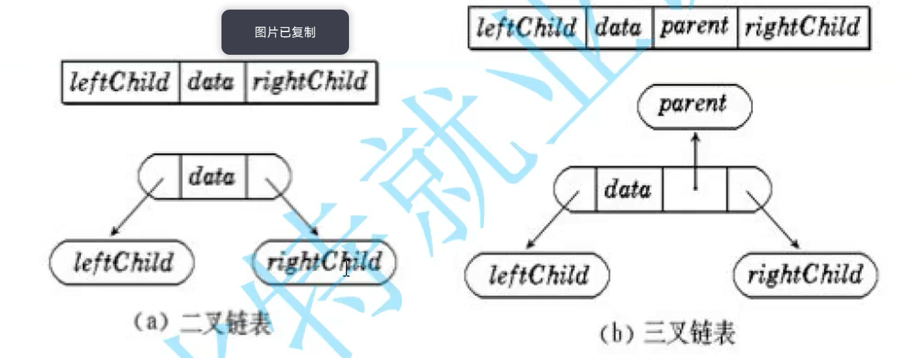
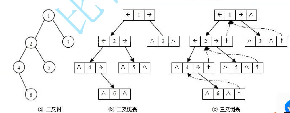
二叉树的链式存储结构是指,用链表来表示一棵二叉树,即用链来指示元素的逻辑关系。通常的方法是链表中每个结点由三个域组成,数据域和左右指针域,左右指针分别用来给出该结点左孩子和右孩子所在的链结点的存储地址。链式结构又分为二叉链和三叉链,当前我们学习中一般都是二叉链,后面课程学到高阶数据结构如红黑树等会用到三叉链。
6.2.4 二叉树的性质
1. 若规定根节点的层数为1,则一棵非空二叉树的第i层上最多有2^(i-1) 个结点。
2. 若规定根节点的层数为1,则深度为h的二叉树的最大结点数是2^h - 1。
3. 对任何一棵二叉树,如果度为0的叶结点个数为 n0,度为2的分支结点个数为 n2,则有n0 = n2 + 1
4. 若规定根节点的层数为1,具有n个结点的满二叉树的深度,h=log2(n + 1)。(ps:log2(n + 1)是log以2为底,n+1为真数)
5. 对于具有n个结点的完全二叉树,如果按照从上至下从左至右的数组顺序对所有节点从0开始编号,则对于序号为i的结点有:
6.3 二叉树的顺序结构及实现
6.3.1 堆的概念及结构
如果有一个关键码的集合K = {k₀, k₁, k₂, …, kₙ₋₁},把它的所有元素按完全二叉树的顺序存储方式存储在一个一维数组中,并满足:Ki ≤ K2 ∗ i + 1 且 Ki ≤ K2 ∗ i + 2(Ki ≥ K2 ∗ i + 1 且 Ki≥ K2 ∗ i + 2),i = 0, 1, 2…,则称为小堆(或大堆)。将根节点最大的堆叫做最大堆或大根堆,根节点最小的堆叫做最小堆或小根堆。
堆的性质:
- 堆中某个节点的值总是不大于或不小于其父节点的值;
- 堆总是一棵完全二叉树。
6.3.2 堆的实现
堆向下调整算法
现在我们给出一个数组,逻辑上看做一颗完全二叉树。我们通过从根节点开始的向下调整算法可以把它调整成一个小堆。向下调整算法有一个前提:左右子树必须是一个堆,才能调整。
//向下调整算法
void AdjustDown(HPDataType* arr, size_t size, int parent)
{
	int child = parent * 2 + 1;
	while (child < size)
	{
		if (child+1<size && arr[child + 1] < arr[child])
		{
			child++;
		}

		if (arr[child] < arr[parent])
		{
			Swap(&arr[child], &arr[parent]);
			parent = child;
			child = parent * 2 + 1;
		}
		else
		{
			break;
		}
	}
}
堆向上调整算法
//向上调整算法
void AdjustUp(HPDataType* arr, int child)
{
	int parent = (child - 1) / 2;

	while (child > 0)
	{
		if (arr[child] < arr[parent])
		{
			Swap(&arr[child], &arr[parent]);
			child = parent;
			parent = (child - 1) / 2;
		}
		else
		{
			break;
		}
	}
}
堆的创建
堆的创建我们可以采用向上调整法或者向下调整法,但是向下调整法的时间复杂度低,效率更高。向下调整算法主要是从倒数的第一个非叶子节点的子树开始调整,一直调整到根节点的树,就可以调整成堆。
//向上调整建堆
for (int i = 1; i < size; i++)
{
	AdjustUp(arr, i);
}

//向下调整建堆
int father = (size - 1 - 1) / 2;
while (father >= 0)
{
	AdjustDown(arr, size, father);
	father--;
}
建堆的时间复杂度
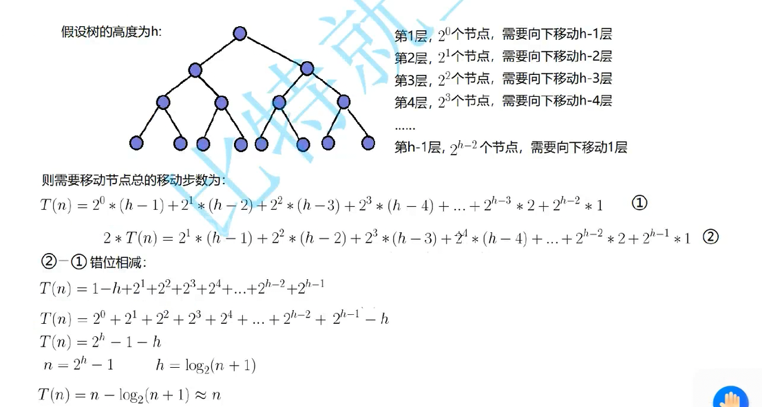
因为堆是完全二叉树,而满二叉树也是完全二叉树,此处为了简化使用满二叉树来证明(时间复杂度本来就是近似值,多几个节点不影响最终结果):
向下调整法的时间复杂度:
向上调整法的时间复杂度:
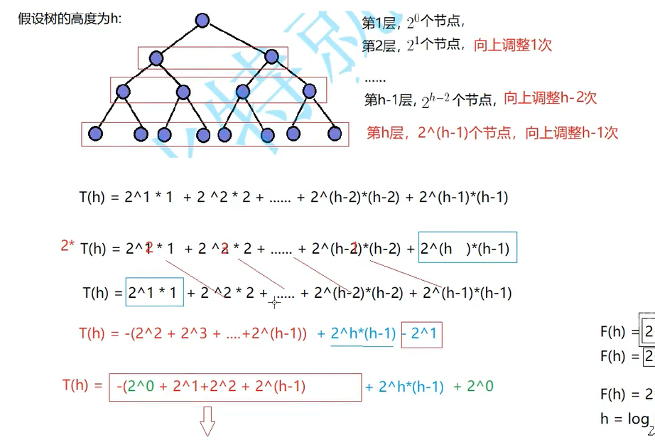
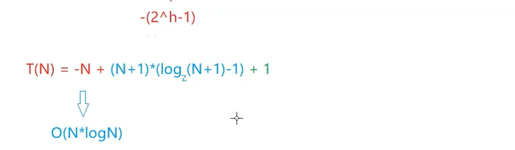
堆的插入
void HPPush(HP* php, HPDataType x)
{
	assert(php);

	if (php->capacity == php->size)
	{
		int newcapacity = php->capacity ? 2 * php->capacity : 4;
		HPDataType* tmp = (HPDataType*)realloc(php->arr, sizeof(HPDataType) * newcapacity);
		if (tmp == NULL)
		{
			perror("realloc");
			exit(EXIT_FAILURE);
		}
		php->arr = tmp;
		php->capacity = newcapacity;
	}

	php->arr[php->size] = x;
	php->size++;

	AdjustUp(php->arr, php->size-1);
}
堆的删除
void HPPop(HP* php)
{
	assert(php && php->arr);

	Swap(&php->arr[0], &php->arr[php->size - 1]);
	php->size--;

	AdjustDown(php->arr, php->size, 0);
}
堆的实现
#define _CRT_SECURE_NO_WARNINGS
#pragma once;
#include<stdbool.h>
#include<stdlib.h>
#include<assert.h>

typedef int HPDataType;

typedef struct Heap
{
	HPDataType* arr;
	int size;
	int capacity;
}HP;

void AdjustUp(HPDataType* arr, int child);

void AdjustDown(HPDataType* arr, size_t size, int parent);

void HPInit(HP* php);

void HPDestroy(HP* php);

void HPPush(HP* php, HPDataType x);

void HPPop(HP* php);

HPDataType HPTop(HP* php);

bool HPEmpty(HP* php);

void Swap(HPDataType* child, HPDataType* parent);
#define _CRT_SECURE_NO_WARNINGS
#include<stdio.h>
#include"BinaryTree.h"
void HPInit(HP* php)
{
assert(php);
php->arr = NULL;
php->capacity = php->size = 0;
}
void HPDestroy(HP* php)
{
assert(php);
free(php->arr);
php->arr = NULL;
php->capacity = php->size = 0;
}
void Swap(HPDataType* child, HPDataType* parent)
{
HPDataType tmp = *child;
*child = *parent;
*parent = tmp;
}
void AdjustUp(HPDataType* arr, int child)
{
int parent = (child - 1) / 2;
while (child > 0)
{
if (arr[child] < arr[parent])
{
Swap(&arr[child], &arr[parent]);
child = parent;
parent = (child - 1) / 2;
}
else
{
break;
}
}
}
void HPPush(HP* php, HPDataType x)
{
assert(php);
if (php->size == php->capacity)
{
int newcapacity = php->capacity ? 2 * php->capacity : 4;
HPDataType* tmp = (HPDataType*)realloc(php->arr, sizeof(HPDataType) * newcapacity);
if (tmp == NULL)
{
perror("realloc");
exit(EXIT_FAILURE);
}
php->arr = tmp;
php->capacity = newcapacity;
}
php->arr[php->size] = x;
php->size++;
AdjustUp(php->arr, php->size - 1);
}
void AdjustDown(HPDataType* arr, size_t size, int parent)
{
int child = parent * 2 + 1;
while (child < size)
{
if (child+1<size && arr[child + 1] < arr[child])
{
child++;
}
if (arr[child] < arr[parent])
{
Swap(&arr[child], &arr[parent]);
parent = child;
child = parent * 2 + 1;
}
else
{
break;
}
}
}
void HPPop(HP* php)
{
assert(php);
assert(php->size);
Swap(&php->arr[0], &php->arr[php->size - 1]);
php->size--;
AdjustDown(php->arr, php->size, 0);
}
HPDataType HPTop(HP* php)
{
assert(php);
assert(php->size);
return php->arr[0];
}
bool HPEmpty(HP* php)
{
assert(php);
return php->size == 0;
}6.3.3 堆的应用
堆排序
- 建堆:首先我们需要根据不同情况来考虑建立大根堆还是小根堆,降序我们选择建立小根堆,升序我们建立大根堆。(我们首先考虑向下调整法建堆,因为向下调整法建堆的时间复杂度更低,这个我们前面提到过)
- 交换首尾节点:我们以降序为例,我们第一次建堆可以得到最小的数(根节点),交换首尾节点相当于把最小的数存在数组的倒数第一个位置,再通过向下调整法调整堆,这样依次得出第二小、第三下的数……并存储好,完成排序。
void HeapSort(int* arr, int size)
{
	//向上调整建堆
	for (int i = 1; i < size; i++)
	{
		AdjustUp(arr, i);
	}

	//向下调整建堆
	int father = (size - 1 - 1) / 2;
	while (father >= 0)
	{
		AdjustDown(arr, size, father);
		father--;
	}

	int end = size;
	while (end--)
	{
		Swap(&arr[end - 1], &arr[0]);
		AdjustDown(arr, end - 1, 0);
	}
}堆排序的时间复杂度为O(nlogn),相较于之前学的冒泡排序(时间复杂度是O(n^2)),时间复杂度小很多,效率也更高。
这个时间复杂度怎么得来的呢?两种情况:向上建堆/向下建堆,在前面我们已经求出,向上 调整法建堆的时间复杂度是O(nlogn),向下调整法建堆的时间复杂度是O(n);后面的排序部分我们不难发现,它的操作过程和向上调整法建堆的过程有异曲同工之妙,时间复杂度为O(nlogn),那么无论是向下调整法建堆还是向上调整法建堆,堆排序的时间复杂度始终为O(nlogn)。
TOP-K 问题
经典OJ算法题:数组中的第K个最大元素
以这道题为例,我们有两种解决办法,最容易想到的一种:堆排序。我们直接用向下调整法建大根堆并排序,轻松得出答案。这个解法的时间复杂度是:建堆O(N)+交换排序O(KlogN)=O(N)。(N远大于K的情况下)
void Swap(int* p1,int* p2)
{
    int tmp=*p1;
    *p1=*p2;
    *p2=tmp;
}

//向下调整法
void AdjustDown(int* nums,int numsSize,int father)
{
    //假设法确定最想子节点的下标
    int child=2*father+1;
    while(child<numsSize)
    {
        if(child+1<numsSize && nums[child+1]>nums[child])
        {
          child++;
        }

        if(nums[child]>nums[father])
        {
           Swap(&nums[child],&nums[father]);
           father=child;
           child=2*father+1;
        }
        else
        {
            break;
        }
    }
}

int findKthLargest(int* nums, int numsSize, int k)
{
    //采用堆排序的办法,向下调整法建堆
    //先取得最后一个非叶子节点的下标
    int father=(numsSize-1-1)/2;
    while(father>=0)
    {
        AdjustDown(nums,numsSize,father);
        father--;
    }

    //把得到的根节点与最后一个叶子节点换位置
    int time=k;
    int fnumsSize=numsSize;
    while(time--)
    {
        Swap(&nums[0],&nums[fnumsSize-1]);
        AdjustDown(nums,--fnumsSize,0);
    }

   return nums[numsSize-k];
}
第二种,我们先建立大小为K的小根堆,再从下标K开始遍历数组,如果遍历到的元素大小大于根节点,那就交换并更新小根堆,继续向后遍历数组。最后小根堆剩下的就是前K个最大元素,轻松得出答案。这个解法的时间复杂度是:建堆O(K)+交换排序O((N-K)logK)=O(N)。两种办法虽然时间复杂度相同,但是第二种解法额外开辟的空间更少,空间复杂度更小,虽然这个题目没有展现出这个优势。
void Swap(int*p1,int*p2)
{
    int tmp=*p1;
    *p1=*p2;
    *p2=tmp;
}

void AdjustDown(int*nums,int numsSize,int father)
{
    //假设法确定最小孩子
    int child=father*2+1;
    while(child<numsSize)
    {
        if(child+1<numsSize&&nums[child+1]<nums[child])
     {
         child++;
     }

    //父亲与孩子开始比比较
     if(nums[father]>nums[child])
     {
         Swap(&nums[father],&nums[child]);
         father=child;
         child=father*2+1;
     }
     else
     {
         break;
     }
    }
}

int findKthLargest(int* nums, int numsSize, int k)
{
   //用前k个元素建小根堆
   int father=(k-1-1)/2;
   int NewNumsSize=k;
   while(father>=0)
   {
     AdjustDown(nums,NewNumsSize,father);
     father--;
   }

   //从下标k处开始遍历原数组,并与根节点比较
   for(int i=k;i<numsSize;i++)
   {
       if(nums[i]>nums[0])
       {
        Swap(&nums[i],&nums[0]);
        AdjustDown(nums,NewNumsSize,0);
       }
   }

   return nums[0];
}
6.4 二叉树链式结构的实现
6.4.2 二叉树的遍历
前序、中序及后序遍历
学习二叉树结构,最简单的方式就是遍历。所谓二叉树遍历 (Traversal) 是按照某种特定的规则,依次对二叉树中的节点进行相应的操作,并且每个节点只操作一次。访问结点所做的操作依赖于具体的应用问题。遍历是二叉树上最重要的运算之一,也是二叉树上进行其它运算的基础。
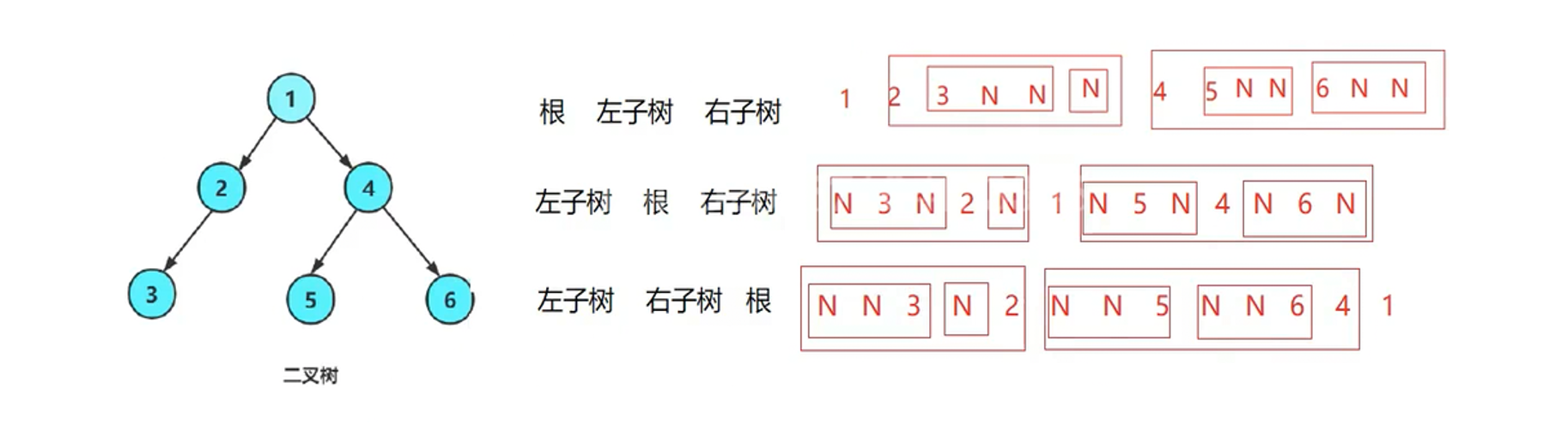
按照规则,二叉树的遍历有:前序/中序/后序的递归结构遍历:
- 前序遍历(Preorder Traversal 亦称先序遍历)——访问根结点的操作发生在遍历其左右子树之前。
- 中序遍历(Inorder Traversal)——访问根结点的操作发生在遍历其左右子树之中(间)。
- 后序遍历(Postorder Traversal)——访问根结点的操作发生在遍历其左右子树之后。
//先序遍历
void PreOrder(BTNode* root)
{
	if (root == NULL)
	{
		printf("N ");
		return;
	}
	printf("%d ", root->x);
	PreOrder(root->left);
	PreOrder(root->right);
}
//中序遍历
void InOrder(BTNode* root)
{
	if (root == NULL)
	{
		printf("N ");
		return;
	}
	InOrder(root->left);
	printf("%d ", root->x);
	InOrder(root->right);
}
//后序遍历
void PostOrder(BTNode* root)
{
	if (root == NULL)
	{
		printf("N ");
		return;
	}
	PostOrder(root->left);
	PostOrder(root->right);
	printf("%d ", root->x);
}
层序遍历
void LevelOrder(BTNode* root)
{
	Queue q1;
	QueueInit(&q1);
	if (root)
	{
		QueuePush(&q1, root);
	}
	while (!QueueEmpty(&q1))
	{
		BTNode* tmp = QueueFront(&q1);
		QueuePop(&q1);
		printf("%d ", tmp->x);
		if (tmp->left)
		{
			QueuePush(&q1, tmp->left);
		}
		if (tmp->right)
		{
			QueuePush(&q1, tmp->right);
		}
	}
	QueueDestroy(&q1);
}
6.4.3 节点个数及高度等
计算节点个数
int TreeSize(BTNode* root)
{
	if (root==NULL)
	{
		return 0;
	}

	return TreeSize(root->left) + TreeSize(root->right)+1;
}
计算叶子节点个数
int TreeLeafSize(BTNode* root)
{
	if (root == NULL)
	{
		return 0;
	}
	if (root->left == NULL && root->right == NULL)
	{
		return 1;
	}

	return TreeLeafSize(root->left) + TreeLeafSize(root->right);
}
计算树的高度
int TreeHigh(BTNode* root)
{
	if (root == NULL)
	{
		return 0;
	}
	int lefthigh = TreeHigh(root->left);
	int righthigh = TreeHigh(root->right);
	return lefthigh > righthigh ? lefthigh + 1 : righthigh + 1;
}
求第K层节点的个数
int TreeLevelKSize(BTNode* root, int k)
{
	if (root == NULL)
	{
		return 0;
	}
	if (k == 1)
	{
		return 1;
	}
	return TreeLevelKSize(root->left, k - 1) + TreeLevelKSize(root->right, k - 1);
}
二叉树查找值为x的节点
BTNode* TreeFind(BTNode* root, BTDataType x)
{
	if (root == NULL)
	{
		return NULL;
	}
	if (root->x == x)
	{
		return root;
	}
	BTNode* ret1 = TreeFind(root->left, x);
	if (ret1)
	{
		return ret1;
	}
	return TreeFind(root->right, x);
}
6.4.4 二叉树OJ题
单值二叉树
相同的树
对称二叉树
另一棵树的子树
6.4.5 二叉树的创建与销毁
二叉树的遍历和创建
二叉树的完全性检验
二叉树的销毁
void TreeDestroy(BTNode* root)
{
	if (root == NULL)
	{
		return;
	}
	TreeDestroy(root->left);
	TreeDestroy(root->right);
	free(root);
}
七. 排序
7.1 常见的排序算法
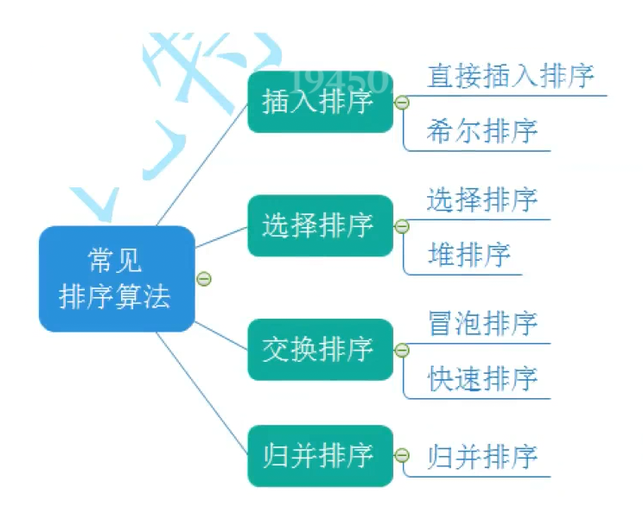
7.2常见排序算法的实现
7.2.1插入排序
直接插入排序
void InsertSort(int* arr, int n)
{
	for (int i = 1; i < n; i++)
	{
		int end = i;
		int tmp = arr[end];
		while (end>0)
		{
			if (arr[end - 1] > tmp)
			{
				arr[end] = arr[end - 1];
				end--;
			}
			else
			{
				break;
			}
		}
		arr[end] = tmp;
	}
}
希尔排序
void ShellSort(int* arr, int n)
{
	int gap = n;
	while (gap > 1)
	{
		gap = gap / 3 + 1;
		for (int i = 0; i < n - gap; i++)
		{
			int end = i;
			int tmp = arr[end + gap];
			while (end >= 0)
			{
				if (arr[end] > tmp)
				{
					arr[end + gap] = arr[end];
					end -= gap;
				}
				else
				{
					break;
				}
			}
			arr[end + gap] = tmp;
		}
	}
}
7.2.2选择排序
选择排序
void SelectSort(int* arr, int n)
{
	int begin = 0;
	int end = n - 1;
	while (begin < end)
	{
		int max = begin;
		int min = begin;

		for (int i = begin+1; i <= end; i++)
		{
			if (arr[i] > arr[max])
			{
				max = i;
			}
			if (arr[i] < arr[min])
			{
				min = i;
			}
		}

		Swap(&arr[min], &arr[begin]);
		if (max == begin)
		{
			max = min;
		}
		Swap(&arr[max], &arr[end]);
		begin++;
		end--;
	}
}
堆排序
void AdjustUp(int* arr, int child)
{
	int father = (child - 1) / 2;
	while (child > 0)
	{
		if (arr[child] < arr[father])
		{
			Swap(&arr[child], &arr[father]);
			child = father;
			father = (child - 1) / 2;
		}
		else
		{
			break;
		}
	}
}

void AdjustDown(int* arr, int father, int n)
{
	int child = 2 * father + 1;
	while (child < n)
	{
		if (child + 1 < n && arr[child + 1] < arr[child])
		{
			child++;
		}

		if (arr[child] < arr[father])
		{
			Swap(&arr[child], &arr[father]);
			father = child;
			child = 2 * father + 1;
		}
		else
		{
			break;
		}
	}
}

void HeapSort(int* arr, int n)
{
	//建堆
    //向上调整法建堆
	for (int i = 1; i < n; i++)
	{
		AdjustUp(arr, i);
	}

	//或者向下调整法建堆(推荐)
	int father = (n - 1 - 1) / 2;
	while (father>=0)
	{
		AdjustDown(arr, father, n);
		father--;
	}

	//排序
	int end = n;
	while (end > 1)
	{
		Swap(&arr[0], &arr[end - 1]);
		AdjustDown(arr, 0, end - 1);
		end--;
	}

}
7.2.3 交换排序
冒泡排序
void BubbleSort(int* arr, int n)
{
	for (int i = 0; i < n - 1; i++)
	{
		int flag = 0;
		for (int j = 0; j < n - i-1; j++)
		{
			if (arr[j] > arr[j + 1])
			{
				flag = 1;
				int tmp = arr[j];
				arr[j] = arr[j + 1];
				arr[j + 1] = tmp;
			}
		}
		if (!flag)
		{
			break;
		}
  }
}
快速排序
int GetMid(int* arr, int left, int right)
{
	int mid = left + (right - left) / 2;
	if (arr[mid] > arr[left])
	{
		if (arr[right] > arr[mid])
		{
			return mid;
		}
		else if (arr[right] > arr[left])
		{
			return right;
		}
		else
		{
			return left;
		}
	}
	else
	{
		if (arr[mid] > arr[right])
		{
			return mid;
		}
		else if (arr[left] < arr[right])
		{
			return left;
		}
		else
		{
			return right;
		}
	}
}

void QuickSortR(int* arr, int left, int right)
{
	ST st;
	STInit(&st);

	STPush(&st,left);
	STPush(&st, right);
	while (!STEmpty(&st))
	{
		int end = STTop(&st);
		STPop(&st);
		int begin = STTop(&st);
		STPop(&st);
		int key = begin;
		int _end = end;
		int _begin = begin;

		while (_begin < _end)
		{
			while (_begin < _end && arr[_end] > arr[key])
			{
				_end--;
			}
			while (_begin < _end && arr[_begin] < arr[key])
			{
				_begin++;
			}
			Swap(&arr[_begin], &arr[_end]);
		}
		Swap(&arr[key], &arr[_begin]);
		key = _begin;

		if (key + 1 < end)
		{
			STPush(&st, key + 1);
			STPush(&st, end);
		}
		if (begin < key - 1)
		{
			STPush(&st, begin);
			STPush(&st, key - 1);
		}
	}

	STDestroy(&st);
}

void QuickSortN(int* arr, int left, int right)
{
	if (left >= right)
	{
		return;
	}

	int prev = left;
	int cur = left + 1;
	int key = left;
	while (cur <= right)
	{
		if (arr[cur] < arr[key]&&++prev!=cur)
		{
			Swap(&arr[prev], &arr[cur]);
		}
		cur++;
	}
	Swap(&arr[prev], &arr[key]);

	QuickSort(arr, left, prev - 1);
	QuickSort(arr, prev + 1, right);
}

void QuickSort(int* arr, int left, int right)
{
	if (left >= right)
	{
		return;
	}

	//小区间优化
	if (right - left + 1 < 10)
	{
		InsertSort(arr + left, right - left + 1);
	}

	//三数取中
	int mid = GetMid(arr, left, right);
	Swap(&arr[mid], &arr[left]);

	int begin = left;
	int end = right;
	int key = left;
	while (begin < end)
	{
		while (begin < end && arr[end] > arr[key] )
		{
			end--;
		}
		while (begin < end && arr[begin] < arr[key])
		{
			begin++;
		}
		Swap(&arr[begin], &arr[end]);
	}
	Swap(&arr[key], &arr[begin]);
	key = begin;
	QuickSort(arr,left ,key-1 );
	QuickSort(arr, key + 1, right);
}
7.2.4 归并排序
void _MergeSort(int* a, int* tmp, int left, int right)
{
	if (left == right)
	{
		return;
	}

	int mid = (left + right ) / 2;
	_MergeSort(a, tmp, left, mid);
	_MergeSort(a, tmp, mid+1, right);

	int begin1 = left;
	int end1 = mid ;
	int begin2 = mid+1;
	int end2 = right;
	int cur = left;

	while (begin1 <= end1 && begin2 <= end2)
	{
		if (a[begin1] <= a[begin2])
		{
			tmp[cur] = a[begin1];
			cur++;
			begin1++;
		}
		else
		{
			tmp[cur] = a[begin2];
			cur++;
			begin2++;
		}
	}

	while (begin1 <= end1)
	{
		tmp[cur] = a[begin1];
		cur++;
		begin1++;
	}

	while (begin2 <= end2)
	{
		tmp[cur] = a[begin2];
		cur++;
		begin2++;
	}
	memcpy(a+left, tmp+left, sizeof(int) * (right - left + 1));
}

void MergeSort(int* a, int n)
{
	int* tmp = (int*)malloc(sizeof(int) * n);
	if (tmp == NULL)
	{
		perror("malloc");
		exit(EXIT_FAILURE);
	}

	_MergeSort(a, tmp, 0, n - 1);

	free(tmp);
	tmp = NULL;
}

void MergeSortR(int* arr, int n)
{
	int* tmp = (int*)malloc(sizeof(int) * n);
	if (tmp == NULL)
	{
		perror("malloc");
		exit(EXIT_FAILURE);
	}

	int gap = 1;
	while (gap < n)
	{
		for (int i = 0; i < n; i += 2 * gap)
		{
			int begin1 = i;
			int end1 = i + gap - 1;
			int begin2 = i + gap;
			int end2 = i + 2 * gap - 1;
			int cur = i;

			if (end1 >= n - 1)
			{
				continue;
			}
			if (begin2 < n && end2 >= n)
			{
				end2 = n - 1;
			}

			while (begin1 <= end1 && begin2 <= end2)
			{
				if (arr[begin1] <= arr[begin2])
				{
					tmp[cur] = arr[begin1];
					cur++;
					begin1++;
				}
				else
				{
					tmp[cur] = arr[begin2];
					cur++;
					begin2++;
				}
			}

			while (begin1 <= end1)
			{
				tmp[cur] = arr[begin1];
				cur++;
				begin1++;
			}

			while (begin2 <= end2)
			{
				tmp[cur] = arr[begin2];
				cur++;
				begin2++;
			}
			memcpy(arr + i, tmp + i, sizeof(int) * (end2 - i + 1));

		}
		gap *= 2;
	}

	free(tmp);
	tmp = NULL;
}
7.2.5 非比较排序(计数排序)
void CountSort(int* arr, int n)
{
	int min = arr[0];
	int max = arr[0];
	for (int i = 0; i < n; i++)
	{
		if (arr[i] > max)
		{
			max = arr[i];
		}
		if (arr[i] < min)
		{
			min = arr[i];
		}
	}

	int numSize = max - min + 1;

	int* tmp = (int*)calloc(numSize, sizeof(int));
	if (tmp == NULL)
	{
		perror("calloc");
		exit(EXIT_FAILURE);
	}

	for (int i = 0; i < n; i++)
	{
		tmp[arr[i] - min]++;
	}

	int cur = 0;
	for (int i = 0; i < numSize; i++)
	{
		while (tmp[i])
		{
			arr[cur] = i + min;
			cur++;
			tmp[i]--;
		}
	}

	free(tmp);
	tmp = NULL;
}
7.3 排序算法复杂度及稳定性分析
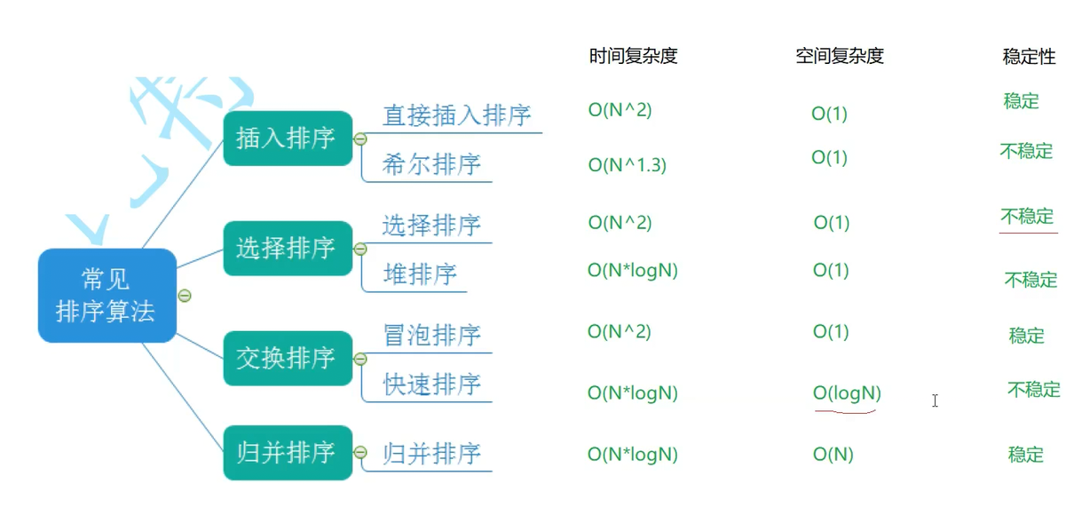
这里解释一下稳定性:相等数值的元素,排序后相对前后位置不变。
更多推荐



 8
8 0
0- 0


 已为社区贡献1条内容

所有评论(0)