import torch

import numpy as np
import pandas as pd
import matplotlib.pyplot as plt

# Rosenbrock function
def f(x):
    return (1 - x[0])**2 + 100 * (x[1] - x[0]**2)**2

def get_grad(y,x):
    # 计算一阶导
    grad = torch.autograd.grad(y, x, retain_graph=True, create_graph=True)
    return grad

# 计算二阶导
def get_hessian(grad,x):
    Hessian = torch.tensor([])
    for anygrad in grad[0]:  # torch.autograd.grad返回的是元组
        Hessian = torch.cat((Hessian, torch.autograd.grad(anygrad, x, retain_graph=True)[0]))
    return (Hessian.view(x.size()[0], -1))

梯度下降法

原理
$x_{n+1}=x_n-\eta g$

lr = 0.001
epochs = 1000
x = torch.tensor([0.5, -1], requires_grad=True)
x0_ls = []
x1_ls = []
y_ls = []

for i in range(epochs):
    y = f(x)
    grad = get_grad(y,x)
    x = x - lr * grad[0]
    
    print(x[0].item(),x[1].item(),y.item())
    x0_ls.append(x[0].item())
    x1_ls.append(x[1].item())
    y_ls.append(y.item())
    

0.25099998712539673 -0.75 156.5
0.17087268829345703 -0.5873997807502747 66.6580581665039
0.1303870975971222 -0.4640803337097168 38.7066650390625
0.10703561455011368 -0.36786410212516785 23.90013313293457
0.09258121252059937 -0.2919999659061432 15.185805320739746
…
0.6774747967720032 0.45742887258529663 0.10440758615732193
0.6777016520500183 0.4577375054359436 0.10426066070795059
0.6779282093048096 0.4580458998680115 0.10411401093006134
0.6781545281410217 0.45835405588150024 0.10396762937307358

# plot the Rosenbrock function
x = np.linspace(-2, 2, 100)
y = np.linspace(-2, 2, 100)
X, Y = np.meshgrid(x, y)
Z = f([X, Y])
plt.contour(X, Y, Z, levels=np.linspace(0, 200, 10))

# plot the path
plt.plot(x0_ls, x1_ls, 'r-')
plt.plot(x0_ls, x1_ls, 'ro')
plt.show()

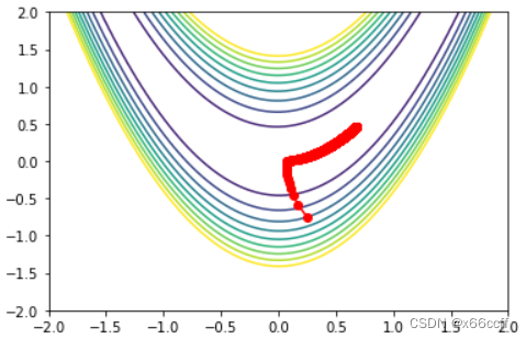
梯度下降法，lr = 0.001 ，迭代了1000步还没到最优点 $(1,1)$，
而 lr 继续增大就会飞出去变成 $(\text{nan},\text{nan})$了

牛顿法

原理：
$x_{n+1}=x_n-H^{-1}g$

lr = 1
epochs = 1000
x = torch.tensor([0.5, -1], requires_grad=True)
x0_ls = []
x1_ls = []
y_ls = []

for i in range(epochs):
    y = f(x)
    grad = get_grad(y,x)
    hessian = get_hessian(grad,x)
    inv_hessian = torch.inverse(hessian)
    x = x - lr * inv_hessian @ grad[0]
    
    print(x[0].item(),x[1].item(),y.item())
    x0_ls.append(x[0].item())
    x1_ls.append(x[1].item())
    y_ls.append(y.item())
    

0.5019919872283936 0.2519921064376831 156.5
0.9996192455291748 0.751605749130249 0.248011976480484
0.9996267557144165 0.999253511428833 6.132203102111816
1.0 0.9999998211860657 1.393127178062059e-07
1.0 1.0 3.197442310920451e-12
…
1.0 1.0 0.0
1.0 1.0 0.0
1.0 1.0 0.0
1.0 1.0 0.0

# plot the Rosenbrock function
x = np.linspace(-2, 2, 100)
y = np.linspace(-2, 2, 100)
X, Y = np.meshgrid(x, y)
Z = f([X, Y])
plt.contour(X, Y, Z, levels=np.linspace(0, 200, 10))

# plot the path
plt.plot(x0_ls, x1_ls, 'r-')
plt.plot(x0_ls, x1_ls, 'ro')
plt.show()

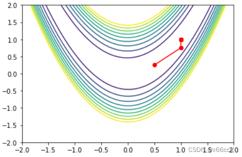
可以看到，牛顿法，设置 lr = 1，只需要4步迭代就达到最优点（初始点未画出），从这里可看出牛顿法的优越性，确实只需要很少的迭代步数就可达到最优点